Evaluation of CFD Methods for Simulation of Two ...

ORNL/TM-2016/612

Evaluation of CFD Methods for Simulation of Two-Phase Boiling Flow Phenomena in a Helical Coil Steam Generator

W. David Pointer, ORNL Dillon Shaver, ANL Yang Liu, ORNL Prasad Vegendla, ANL Adrian Tentner, ANL September 30, 2016

Approved for public release. Distribution is unlimited.

DOCUMENT AVAILABILITY Reports produced after January 1, 1996, are generally available free via US Department of Energy (DOE) SciTech Connect. Website http://www.osti.gov/scitech/ Reports produced before January 1, 1996, may be purchased by members of the public from the following source: National Technical Information Service 5285 Port Royal Road Springfield, VA 22161 Telephone 703-605-6000 (1-800-553-6847) TDD 703-487-4639 Fax 703-605-6900 E-mail [email protected] Website http://www.ntis.gov/help/ordermethods.aspx Reports are available to DOE employees, DOE contractors, Energy Technology Data Exchange representatives, and International Nuclear Information System representatives from the following source: Office of Scientific and Technical Information PO Box 62 Oak Ridge, TN 37831 Telephone 865-576-8401 Fax 865-576-5728 E-mail [email protected] Website http://www.osti.gov/contact.html

This report was prepared as an account of work sponsored by an agency of the United States Government. Neither the United States Government nor any agency thereof, nor any of their employees, makes any warranty, express or implied, or assumes any legal liability or responsibility for the accuracy, completeness, or usefulness of any information, apparatus, product, or process disclosed, or represents that its use would not infringe privately owned rights. Reference herein to any specific commercial product, process, or service by trade name, trademark, manufacturer, or otherwise, does not necessarily constitute or imply its endorsement, recommendation, or favoring by the United States Government or any agency thereof. The views and opinions of authors expressed herein do not necessarily state or reflect those of the United States Government or any agency thereof.

ORNL/TM-2016/612

Reactor and Nuclear Systems Division

Evaluation of CFD Methods for Simulation of Two-Phase Boiling Flow Phenomena in a Helical Coil Steam Generator W. David Pointer, Oak Ridge National Laboratory Dillon Shaver, Argonne National Laboratory Yang Liu, Oak Ridge National Laboratory Prasad Vegendla, Argonne National Laboratory Adrian Tentner, Argonne National Laboratory

Date Published: September 30, 2016

Prepared by OAK RIDGE NATIONAL LABORATORY Oak Ridge, TN 37831-6283 managed by UT-BATTELLE, LLC for the US DEPARTMENT OF ENERGY under contract DE-AC05-00OR22725

CONTENTS

LIST OF FIGURES ............................................................................................................................... IV LIST OF TABLES ................................................................................................................................ VI ACRONYMS........................................................................................................................................7 ABSTRACT ..........................................................................................................................................8 1.

INTRODUCTION ..........................................................................................................................9 1.1 INDUSTRY APPLICATION....................................................................................................................... 9 1.2 BASIS FOR METHODOLOGY DEMONSTRATIONS ........................................................................................ 9 1.2.1 Geometry .............................................................................................................................10 1.2.2 Boundary Conditions ............................................................................................................10 1.2.3 Measurements .....................................................................................................................11

2.

CFD CODES APPLIED .................................................................................................................. 12 2.1 STAR-CCM+ ..................................................................................................................................12 2.2 NEK5000 .......................................................................................................................................13

3.

COMPUTATIONAL MODELS ....................................................................................................... 17 3.1 STAR-CCM+ ..................................................................................................................................17 3.2 COMPUTATIONAL MESH DEVELOPMENT ..............................................................................................17 3.3 BENCHMARKING SINGLE PHASE STAR-CCM+ PREDICTIONS ...................................................................23 3.3.1 Nek5000 ...............................................................................................................................24

4.

LAMINAR SINGLE PHASE FLOW SIMULATIONS ........................................................................... 27 4.1 NEK5000 SIMULATIONS ....................................................................................................................27 4.2 STAR-CCM+ SIMULATIONS ...............................................................................................................28 4.3 NEK5000 VS. STAR-CCM+ BENCHMARKING .......................................................................................29

5.

TURBULENT MULTIPHASE FLOW SIMULATIONS ......................................................................... 30 5.1 MULTIPHASE MIXTURE MODEL SIMULATIONS ........................................................................................30 5.1.1 Simplified Turbulence Model in Nek5000 ............................................................................30 5.1.2 The Regularized κ-ω Model in Nek5000 ..............................................................................32 5.2 EULERIAN-EULERIAN SIMULATIONS .....................................................................................................33 5.2.1 Baseline Multi-Phase Closure Models ..................................................................................33 5.2.2 Sensitivity to Closure Models ...............................................................................................37 5.2.3 Sensitivity to wall heat boundary conditions .......................................................................39 5.2.4 Sensitivity to flow rate .........................................................................................................40 5.3 TWO-PHASE BOILING FLOW BENCHMARKING .......................................................................................42 5.4 NEK5000 VS. STAR-CCM+ COMPARISONS .........................................................................................43

6.

FUTURE WORK ......................................................................................................................... 44

7.

CONCLUSIONS .......................................................................................................................... 45

REFERENCES .................................................................................................................................... 46

iii

LIST OF FIGURES FIG. 1 GEOMETRIC CONFIGURATION CONSIDERED IN ASSESSMENT OF METHODOLOGY APPLICABILITY. ............................................... 10 FIG. 2. MIXTURE PROPERTY MODELS SHOWING (A) DENSITY AND (B) MODIFIED VOLUME EXPANSION COEFFICIENT ACROSS THE COMPLETE MODEL RANGE AND (C) DENSITY AND (D) MODIFIED VOLUME EXPANSION COEFFICIENT ACROSS A NARROW RANGE CENTERED AT THE LIQUID-TO-TWO-PHASE TRANSITION............................................................................................................................. 16 FIG. 3. CROSS SECTIONAL DISTRIBUTION OF COMPUTATIONAL MESH WITH WELL RESOLVED BOUNDARY LAYER. ................................... 18 FIG. 4. PREDICTED VELOCITY PROFILE IN THE REFERENCE SIMULATION USING THE LOW REYNOLDS NUMBER VARIANT OF THE REALIZABLE KEPSILON TURBULENCE MODEL. SECONDARY FLOW STRUCTURE IS HIGHLIGHTED BY THE LINE INTEGRAL CONVOLUTION. ................. 18 FIG. 5. PREDICTED DIFFERENTIAL PRESSURE DISTRIBUTION IN THE REFERENCE SIMULATION USING THE LOW REYNOLDS NUMBER VARIANT OF THE REALIZABLE K-EPSILON TURBULENCE MODEL............................................................................................................. 19 FIG. 6. COMPUTATIONAL MESHES USED IN MESH SENSITIVITY STUDY: (A) NOMINAL POLYHEDRAL CORE MESH, (B) POLYHEDRAL CORE MESH WITH EXTENDED PRISMATIC EXTRUSION LAYER, (C) NOMINAL HEXAHEDRAL BLOCK-STRUCTURED MESH, AND (D) REFERENCE WALLREFINED HEXAHEDRAL BLOCK-STRUCTURED MESH. .......................................................................................................... 20 FIG. 7. PREDICTED VELOCITY PROFILES ALONG THE HORIZONTAL TUBE DIAMETER FOR 3 ALTERNATE COMPUTATIONAL MESH CONFIGURATIONS AND THE REFERENCE LOW Y+ SIMULATION. DATA ARE EXTRACTED IN THE CROSS SECTION LOCATED 1½ REVOLUTIONS OF THE HELICAL PIPE FROM THE INLET........................................................................................................ 21 FIG. 8. EVOLUTION OF PREDICTED VELOCITY PROFILES ALONG THE HORIZONTAL PIPE DIAMETER AS COOLANT MOVES THROUGH THE HELIX. ............................................................................................................................................................................. 22 FIG. 9. PREDICTED VELOCITY PROFILE IN THE REFERENCE SIMULATION USING THE HIGH REYNOLDS NUMBER VARIANT OF THE REALIZABLE KEPSILON TURBULENCE MODEL. SECONDARY FLOW STRUCTURE IS HIGHLIGHTED BY THE LINE INTEGRAL CONVOLUTION. ................. 22 FIG. 10. PREDICTED DIFFERENTIAL PRESSURE DISTRIBUTION IN THE REFERENCE SIMULATION USING THE HIGH REYNOLDS NUMBER VARIANT OF THE REALIZABLE K-EPSILON TURBULENCE MODEL. ....................................................................................................... 23 FIG. 11. COMPARISON OF CFD PREDICTIONS OF SINGLE-PHASE PRESSURE DROP WITH THREE EXPERIMENTAL CORRELATIONS................ 24 FIG. 12. CROSS SECTION VIEWS OF THE MESHES USED IN THE INITIAL NEK5000 SIMULATIONS OF THE HELICAL COIL SHOWING THE INITIAL MESH GENERATED WITH STAR-CCM+ AND THE MESH GENERATED USING PRENEK. IMAGES SHOW BOTH ELEMENT BOUNDARIES AND GAUSS-LOBATTO-LEGENDRE POINTS ASSOCIATED WITH THE HIGHER ORDER SPECTRAL SOLUTION. ........................................... 25 FIG. 13 THE MESH GENERATED FOR USE WITH THE Κ-Ω MODEL IN NEK5000 SHOWING THE CROSS SECTION VIEW AND THE MESH REFINEMENT CLOSE TO THE WALL................................................................................................................................. 26 FIG. 14. CROSS SECTIONAL SLICES AT ½ ROTATION FROM THE INLET FOR THE LAMINAR, SINGLE PHASE NEK5000 SIMULATION SHOWING (A) THE AXIAL VELOCITY WITH OVERLAID TRANSVERSE VECTORS, (B) THE TRANSVERSE VELOCITY MAGNITUDE, AND (C) THE SUBCOOLING. THE CENTER OF THE HELIX IS ON THE RIGHT IN ALL THREE IMAGES....................................................................................... 27 FIG. 15. CROSS SECTIONAL SLICES AT 1 FULL ROTATION FROM THE INLET FOR THE LAMINAR, SINGLE PHASE NEK5000 SIMULATION SHOWING (A) THE AXIAL VELOCITY WITH OVERLAID TRANSVERSE VECTORS, (B) THE TRANSVERSE VELOCITY MAGNITUDE, AND (C) THE SUBCOOLING. THE CENTER OF THE HELIX IS ON THE RIGHT IN ALL THREE IMAGES. .................................................................. 28 FIG. 16. CROSS SECTIONAL SLICES AT 1 FULL ROTATION FROM THE INLET FOR THE LAMINAR, SINGLE PHASE STAR-CCM+ SIMULATION SHOWING (A) THE AXIAL VELOCITY WITH OVERLAID TRANSVERSE VECTORS, (B) THE TRANSVERSE VELOCITY MAGNITUDE, AND (C) THE SUBCOOLING. THE CENTER OF THE HELIX IS ON THE RIGHT IN ALL THREE IMAGES. .................................................................. 28 FIG. 17. CROSS SECTIONAL SLICES AT 1¼ ROTATIONS FROM THE INLET FOR THE SIMPLIFIED TURBULENCE MODEL WITH THE HEM FORMULATION SHOWING THE AXIAL MIXTURE VELOCITY OVERLAID WITH TRANSVERSE VELOCITY VECTORS, THE MAGNITUDE OF THE TRANSVERSE VELOCITY, THE MIXTURE SUBCOOLING, AND THE VAPOR PHASE VOLUME FRACTION. EACH ROW SHOWS RESULTS FROM A SIMULATION USING THE IDENTIFIED TURBULENCE MULTIPLIER. .......................................................................................... 31 FIG. 18. CROSS SECTIONAL SLICES AT 1½ ROTATIONS FROM THE INLET FOR THE SIMPLIFIED TURBULENCE MODEL WITH THE HEM FORMULATION SHOWING THE AXIAL MIXTURE VELOCITY OVERLAID WITH TRANSVERSE VELOCITY VECTORS AND THE VAPOR PHASE VOLUME FRACTION. EACH ROW SHOWS RESULTS FROM A SIMULATION USING THE IDENTIFIED TURBULENCE MULTIPLIER. ............. 31

FIG. 19. CROSS SECTIONAL SLICES AT 1¼ ROTATIONS FROM THE INLET FOR THE Κ-Ω TURBULENCE MODEL WITH THE HEM FORMULATION SHOWING THE AXIAL MIXTURE VELOCITY OVERLAID WITH TRANSVERSE VELOCITY VECTORS, THE MIXTURE SUBCOOLING, AND THE VAPOR PHASE VOLUME FRACTION. ............................................................................................................................... 32 FIG. 20. CROSS SECTIONAL SLICES AT 1¼ ROTATIONS FROM THE INLET FOR THE Κ-Ω TURBULENCE MODEL WITH THE HEM FORMULATION SHOWING THE TURBULENT KINETIC ENERGY, THE TURBULENCE DISSIPATION FREQUENCY (Ω), AND THE RATIO OF EDDY VISCOSITY TO LAMINAR VISCOSITY................................................................................................................................................... 32

iv

FIG. 21. EVOLUTION OF TEMPERATURE PROFILE IN THE HELICAL COIL STEAM GENERATOR TUBE USING THE BASELINE MODEL CONFIGURATION. THE CENTER OF THE HELIX IS ON THE RIGHT IN ALL IMAGES. A POLAR COORDINATE NOTATION IS USED TO INDICATE POSITION IN THE HELIX, WITH 2INDICATING ONE FULL ROTATION AROUND THE HELIX. ......................................................... 36 FIG. 22. EVOLUTION OF VAPOR DISTRIBUTION IN THE HELICAL COIL STEAM GENERATOR TUBE USING THE BASELINE MODEL CONFIGURATION. THE CENTER OF THE HELIX IS ON THE RIGHT IN ALL IMAGES. A POLAR COORDINATE NOTATION IS USED TO INDICATE POSITION IN THE HELIX, WITH 2INDICATING ONE FULL ROTATION AROUND THE HELIX................................................................................. 36 FIG. 23. SECONDARY FLOW FIELD IN THE HELICAL COIL STEAM GENERATOR TUBE AFTER 1¼ REVOLUTIONS (2½ IN THE POLAR COORDINATE NOTATION) AROUND THE HELIX FOR BOTH SINGLE AND TWO-PHASE FLOW. THE CENTER OF THE HELIX IS ON THE RIGHT IN ALL IMAGES.......................................................................................................................................................... 37 FIG. 24. COMPARISON OF BASELINE SIMULATION RESULTS (TOMIYAMA MODEL) WITH TWO ALTERNATE DRAG COEFFICIENT MODELS IN THE CROSS SECTION AFTER THE FLOW HAS COMPLETED 1½ ROTATIONS (3 IN POLAR COORDINATE SYSTEM NOTATION). PREDICTED AXIAL VELOCITY OF THE LIQUID PHASE WITH TRANSVERSE FLOW STRUCTURES ARE SHOWN, HIGHLIGHTED WITH THE LINE INTEGRAL CONVOLUTION, PREDICTED TEMPERATURE DISTRIBUTION, PREDICTED VOID DISTRIBUTION AND PREDICTED SAUTER MEAN BUBBLE DIAMETER. .............................................................................................................................................................. 38 FIG. 25. PREDICTED VOID FRACTIONS IN TWO COMPARABLE CASES WITH CONSTANT WALL TEMPERATURE (TOP ROW) AND CONSTANT WALL HEAT FLUX (BOTTOM ROW). THE CENTER OF THE HELIX IS TO THE RIGHT IN ALL IMAGES. A POLAR COORDINATE NOTATION IS USED TO INDICATE POSITION IN THE HELIX, WITH 2INDICATING ONE FULL ROTATION AROUND THE HELIX. ............................................ 39 FIG. 26. PREDICTED SAUTER MEAN BUBBLE DIAMETER IN TWO COMPARABLE CASES WITH CONSTANT WALL TEMPERATURE (TOP ROW) AND CONSTANT WALL HEAT FLUX (BOTTOM ROW). THE CENTER OF THE HELIX IS TO THE RIGHT IN ALL IMAGES. A POLAR COORDINATE NOTATION IS USED TO INDICATE POSITION IN THE HELIX, WITH 2INDICATING ONE FULL ROTATION AROUND THE HELIX. .............. 40 FIG. 27. COMPARISON OF BASELINE SIMULATION RESULTS WITH TWO ALTERNATE BOUNDARY CONDITION SETS IN THE CROSS SECTION AFTER THE FLOW HAS COMPLETED 1½ ROTATIONS (3 IN POLAR COORDINATE SYSTEM NOTATION). DIFFERENCES IN FLOW RATE ARE NOTED; POWER-TO-FLOW RATIOS WERE MAINTAINED. SHOWN ARE PREDICTED AXIAL VELOCITY WITH TRANSVERSE FLOW STRUCTURES HIGHLIGHTED WITH THE LINE INTEGRAL CONVOLUTION, PREDICTED TEMPERATURE DISTRIBUTION, PREDICTED VOID DISTRIBUTION AND PREDICTED SAUTER MEAN BUBBLE DIAMETER................................................................................................................. 41 FIG. 28. COMPARISON OF PREDICTED TWO-PHASE PRESSURE DROPS FROM CFD SIMULATIONS AND TWO CORRELATIONS. ................... 43 FIG. 29. COMPARISON OF PREDICTED VOID FRACTION DISTRIBUTIONS AFTER THE FLUID HAS MOVED THROUGH 1¼ ROTATIONS OF THE HELICAL COIL FROM NEK5000 MIXTURE MODEL (LEFT) AND STAR-CCM+ EULERIAN-EULERIAN TWO-FLUID SIMULATIONS (RIGHT). ............................................................................................................................................................................. 43

v

LIST OF TABLES TABLE 1. FACILITY DIMENSIONS............................................................................................................................................ 10 TABLE 2. CONDITIONS CONSIDERED IN EXPERIMENTS AND SIMULATIONS...................................................................................... 11

vi

ACRONYMS ALCF ANSYS ICEM CFD CASL CFD DC DFM DOE DOE-NE GLL HEM HIP HTGR LES LWR MPI NEAMS Nek5000 OLCF RANS SFR SGFIV SIMPLE SMR STAR-CCM+ 2P2F

Argonne Leadership Computing Facility [not an acronym; commercial software package] computational fluid dynamics Consortium for Advanced Simulation of Light Water Reactors computational fluid dynamics direct current drift flux model US Department of Energy Department of Energy Office of Nuclear Energy Gauss-Lobatto-Legendre homogeneous equilibrium model high impact problem high temperature gas-cooled reactor large eddy simulation light water reactor message passing interface Nuclear Energy Advanced Modeling and Simulation [not an acronym, open source code] Oak Ridge Leadership Computing Facility Reynolds Averaged Navier Stokes sodium-cooled fast reactor steam generator flow induced vibration Semi-Implicit Method for Pressure-Linked Equations small modular reactor [not an acronym, commercial simulation software] two-phase two-fluid

7

ABSTRACT The US Department of Energy’s Office of Nuclear Energy charges participants in the Nuclear Energy Advanced Modeling and Simulation (NEAMS) program with developing advanced modeling and simulation capabilities to address design, performance, and safety challenges in the development and deployment of advanced reactor technology. NEAMS has established a high impact problem (HIP) team to demonstrate how these tools can be used to identify and mitigate sources of steam generator flow induced vibration (SGFIV). The SGFIV HIP team is evaluating vibration sources in an advanced helical coil steam generator using:  computational fluid dynamics (CFD) simulations of the turbulent primary coolant flow over the outside of the tubes, and  CFD simulations of the turbulent multiphase boiling secondary coolant flow inside the tubes integrated with high resolution finite element method assessments of the tubes and their associated structural supports. This report summarizes the demonstration of a methodology for multiphase boiling flow analysis inside the helical coil steam generator tube. A helical coil steam generator configuration has been defined based on the experiments completed by Polytecnico di Milano in the SIET helical coil steam generator tube facility. Simulations of the defined problem have been completed using the Eulerian-Eulerian multi-fluid modeling capabilities of the commercial CFD code STAR-CCM+. Simulations suggest that the two phases will quickly stratify in the slightly inclined pipe of the helical coil steam generator. These results have been successfully benchmarked against both empirical correlations for pressure drop and simulations using an alternate CFD methodology, the dispersed phase mixture modeling capabilities of the open source CFD code Nek5000.

8

1.

INTRODUCTION

The Nuclear Energy Advanced Modeling and Simulation Program (NEAMS) program, carried out under the auspices of the US Department of Energy’s Office of Nuclear Energy (DOE-NE), established two high impact problem (HIP) teams in March 2015. The NEAMS HIP teams were challenged to identify a problem of high importance to the nuclear power industry and demonstrate the impact of the NEAMS high performance modeling and simulation tools by providing innovative solutions to those problems. The teams were further challenged to establish a collaborative relationship with an end customer for this solution in industry or for more application-focused DOE-NE programs that would ultimately evaluate the success or failure of the HIP team solution. One of the two HIP teams is focused on demonstrating capabilities to address challenges in the design and development of long-life helical coil steam generators for application in advanced small modular nuclear reactors (SMRs). In particular, this HIP team seeks to address structural restraint design requirements for the helical coil steam generator to mitigate risk from Steam Generator Flow Induced Vibration (SGFIV). The HIP team is evaluating capabilities to predict the structural impacts of vibrations induced by (1) the single-phase liquid primary system coolant flowing over the outside of the tubes and (2) by the boiling multiphase secondary system coolant flowing through the inside of the tubes. This report summarizes the assessment of the applicability of multi-phase boiling simulation technologies to evaluations of the steam generator secondary side. 1.1

INDUSTRY APPLICATION

Many integral SMR designs rely on natural convection rather than forced flow from a pump to drive the flow of primary coolant through the reactor and associated heat removal systems, while secondary loop steam cycle systems include feedwater pumps to control steam generator levels and steam production rates. Helical coil steam generators are widely used as an off-the-shelf technology in industrial applications because they have good pressure drop and heat transfer coefficient characteristics. They have been applied in many historical nuclear reactors, including the Otto Hahn nuclear ship, the SuperPhoenix sodium-cooled fast reactor (SFR) and the Fort St. Vrain High Temperature Gas-cooled Reactor (HTGR). The helical coil footprint, which can tightly encircle the reactor core, is especially amenable to application within integral SMR concepts in which all components that contact the primary coolant are enclosed within the reactor vessel. In integral SMR applications, the primary coolant typically flows over the outside of the steam generator tubes, and boiling secondary flow coolant typically flows through the inside of the steam generator tubes. This configuration optimizes pressure drops in the primary coolant loop to provide maximum natural convection flow and heat removal during postulated accident scenarios. 1.2

BASIS FOR METHODOLOGY DEMONSTRATIONS

Rather than addressing a particular steam generator design, this assessment of code applicability for evaluations of boiling flows inside the steam generator tube addresses the configuration evaluated in published experiments executed by Politecnico di Milano [1,2] at the SIET laboratory [3] in Piacenza, Italy. The test section is fed from a large tank of demineralized water by a centrifugal booster pump in series with a feed-water pump driven by an asynchronous three-phase motor. Flow rate is controlled by opening or closing a control valve to a bypass line which returns to a tank. A throttling valve before the test section provides a large pressure drop to reduce to the likelihood of flow instability in the test section when powered. The coolant passes through a coiled tube preheater before it enters the test section to provide control of inlet temperature conditions. A direct current (DC) is applied to the test section, and it is directly heated by Joule heating.

9

1.2.1

Geometry

The test section geometry is illustrated in a notional diagram in Fig. 1. Dimensions are given in Table 1. Most simulations in this applicability assessment address only the first two rotations of the helical coil in order to reduce computational burden and focus on the evolution of the interface between liquid and gas phases in the pipe.

Coil Pitch

Height

Dcoil Fig. 1 Geometric configuration considered in assessment of methodology applicability.

Table 1. Facility dimensions.

Inner tube diameter, d (mm) Outer tube diameter (mm) Coil diameter, D (mm) Coil pitch (mm) Tube length, total (m) Steam generator height (m)

1.2.2

12.53 17.24 1000 800 32 8

Boundary Conditions

Experiments in the SIET facility cover a wide range of conditions that might be experienced in the steam generator. The range of conditions considered is summarized in Table 2. The actual conditions for the final application of the modeling strategy developed in these studies are not yet known, as they will be defined by the identified customer in the final year of the effort. In these studies, which include parametric assessments of model sensitivities, a nominal case has been defined, as shown in Table 2. Conditions near the upper limit of those considered in the experiment were selected so that most of the liquid coolant would be converted to vapor by the end of the helical coil’s two rotations as addressed in the nominal model.

10

Table 2. Conditions considered in experiments and simulations.

1.2.3

Boundary Condition

Range in experiments [2]

Nominal value in simulations

Mass flux (kg/m2s) Pressure (bar) Thermal flux (kW/m2) Subcooling (K) Diameter ratio, D/d

192 – 811 11 – 63 50 – 200 15-75 79.8

800 60 150 50 79.8

Measurements

The experiments completed in the SIET helical coil boiling facility were focused on developing appropriate engineering correlations for pressure drop and heat transfer coefficient to be used in reducedorder lumped-parameter codes. Flow rate is measured before the flow enters the preheater so that flow rates are recorded at the coolant density associated with the room temperature tank. Therefore, flow rates should be converted to inlet velocities using room temperature properties. Coolant temperatures are measured via thermocouples at the inlet outlet and an intermediate position. Absolute pressures are measured at the inlet and outlet. Differential pressures are measured at the same position, corresponding to a rotation angle of /2 from the inlet, in each loop of the helical coil. Total power consumed by the heated test section is measured at the power supply. Exit qualities are calculated based on energy balance. No detailed measurements of velocity, temperature, or vapor distributions are included in the experiments.

11

2.

CFD CODES APPLIED

In the evaluation of SGFIV phenomena in helical coil steam generators, analysts must be able to define both the expected distribution of vapor within the steam generator tubes and the local boiling conditions within the tubes that define the direct vibration contributions from the boiling itself. In the former case, the density distribution of the material within the tube must be known in order to properly account for damping of vibrations by the secondary side coolant. In the latter case, local parameters such as coolant temperature, bubble formation rates, bubble departure rates, and vapor distribution in the cross section must be known in order to estimate vibration contributions from the boiling flow. In this study, two distinctly different multiphase simulation capabilities are being used to evaluate the boiling secondary side flow inside the steam generator tube. STAR-CCM+ [4] is a commercial CFD code which serves as the principal development platform for advanced multiphase flow boiling models in the Consortium for Advanced Simulation of Light Water Reactors (CASL), a US DOE program focused on developing integrated multiphysics modeling and simulation capabilities for the conventional fleet of light water reactors (LWRs). Nek5000 is a highly scalable open source CFD code which serves as the principal development platform for thermal fluid analysis capabilities in the NEAMS program. The developing capabilities of the multiphase flow version of the Nek5000 code are used as a benchmarking capability for the more mature multiphase flow capabilities of the STAR-CCM+ code. 2.1

STAR-CCM+

The commercial CFD code STAR-CCM+ is a general-purpose analysis package for thermal and compressible/incompressible fluid flow phenomena based on the finite volume formulation. STARCCM+ supports the use of generic polyhedral mesh elements and provides multiple approaches for fully parallel generation of conformal computational meshes describing complex geometries. The code provides capabilities for Reynolds Averaged Navier Stokes (RANS) modeling and Large Eddy Simulation (LES). All simulations presented in this report use  type RANS turbulence models. Solutions are obtained via the SIMPLE algorithm with Rhie-Chow interpolation for velocity to pressure coupling. Solutions are accelerated with algebraic multi-grid preconditioning. Energy to flow coupling is treated using a split operator methodology. The code provides second order accuracy in its resolution of spatial and temporal phenomena. However, all calculations in the present study are steady state. STAR-CCM+ includes several features for multiphase flow analysis, including volume of fluid methods, Lagrangian particle tracking methods, Eulerian multiphase mixture models such as the homogeneous equilibrium model (HEM) and the drift flux model (DFM), and Eulerian-Eulerian dispersed phase models. The Eulerian-Eulerian dispersed phase models serve as the foundation for the CASL program’s development of an advanced boiling simulation capability. More details of CASL’s development efforts with the Eulerian-Eulerian CASL closure model can be found in Reference 4. The Eulerian-Eulerian dispersed phase model is implemented as an n-fluid n-field model with the following conservations equations given as 𝜕 (𝛼𝑘 𝜌𝑘 ) + 𝜕𝑡 𝜕 𝜕𝑡

𝛁 ∙ (𝛼𝑘 𝜌𝑘 𝒖𝑘 ) = (𝑚̇𝑘𝑖 − 𝑚̇𝑖𝑘 ),

(𝛼𝑘 𝜌𝑘 𝒖𝑘 ) + 𝜵 ∙ (𝛼𝑘 𝜌𝑘 𝒖𝑘 𝒖𝑘 ) − 𝜵 ∙ (𝛼𝑘 (𝝉𝑘 − 𝝉𝑘 ′)) = 𝛼𝑘 𝛻𝑝 + 𝛼𝑘 𝜌𝑘 𝒈 + 𝑴, and

12

(1) (2)

𝜕 (𝛼 𝜌 𝑒 ) + 𝜵 ∙ (𝛼𝑘 𝜌𝑘 𝒖𝑘 𝑒𝑘 ) − 𝜵 ∙ (𝛼𝑘 𝜆𝑘 ∇𝑇𝑘 ) = 𝑄, 𝜕𝑡 𝑘 𝑘 𝑘

(3)

𝑀 = 𝐹𝐷𝑟𝑎𝑔 + 𝐹𝐿𝑖𝑓𝑡 + 𝐹𝑇𝑢𝑟𝑏.𝐷𝑖𝑠𝑝. + 𝐹𝑊𝑎𝑙𝑙 𝐿𝑢𝑏. + 𝐹𝑉𝑖𝑟𝑡.𝑀𝑎𝑠𝑠 + 𝑚̇𝑘𝑖 𝑢𝑖 − 𝑚̇𝑖𝑘 𝑢𝑘 .

(4)

where

The conservation equations above are written for phase k such that 𝛼𝑘 is the volume fraction of phase k, and 𝑚̇𝑘𝑖 is the mass transfer rate from phase k to phase i. Closure models are selected by the user to describe each force term that acts on the dispersed phase bubbles or droplets. Additionally, a wall heat partitioning model is implemented to describe the transfer of heat from the wall to the coolant. The heat flux from the wall to the liquid is divided into three parts: convective heat transfer to the liquid, evaporative heat transfers for generation of steam, and quenching heat transfer for heating of liquid in the nucleation sites as the bubble departs. The convergence criterion for STAR-CCM+ was defined as the reduction of all conservation equation residuals by 4 orders of magnitude, or reducing the normalized residuals below 10 -4. However, residual normalization can be deceptive in two-phase simulations because they are typically initialized with single-phase flow conditions. Therefore, asymptotic convergence of void fraction and flow conditions should also be tracked at selected monitoring points. 2.2

NEK5000

Nek5000 is an open source spectral element CFD code originally developed for high-fidelity simulations of turbulence phenomena in single-phase flows, typically focused on the LES or direct numerical simulation classes of CFD. Written in classical FORTRAN, it is a massively parallel code implemented with message passing interface (MPI), and it has been demonstrated at leadership class computing facilities, including the Argonne Leadership Computing Facility (ALCF) and Oak Ridge Leadership Computing Facility (OLCF). Recently, a two-phase flow capability has been implemented in the Nek5000 version referred to as NEK-2P. Significant efforts have also been focused on development of RANS-type turbulence models, specifically a novel variant of a two-equation RANS model, the 𝜅-𝜔 model. Development of the RANS capability in Nek5000 includes the formulation and implementation of a novel regularized 𝜅-𝜔 model as described by Tomboulides et al. [6]. A typical 𝜅-𝜔 model requires a numerical approximation of infinity as a wall boundary condition in the 𝜔 equation. This type of approach is difficult to implement with a high fidelity code such as Nek5000 in which the wall boundary points are solved explicitly. By reformulating the model so that the asymptotic near-wall behavior of 𝜔 is treated analytically, a new equation for 𝜔 has been formulated which can be implemented in a stable manner. The typical governing equations for the 𝜅-𝜔 model are given as 𝐷𝜅 𝜇 ⃗ ⋅ [(𝜇 + 𝑡 ) ∇ ⃗ 𝜅] + 𝐺𝜅 − 𝑌𝜅 =∇ 𝐷𝑡 𝜎𝜅 𝐷𝜔 𝜇 ⃗ ⋅ [(𝜇 + 𝑡 ) ∇ ⃗ 𝜔] + 𝐺𝜔 − 𝑌𝜔 𝜌 =∇ 𝐷𝑡 𝜎𝜔 𝜌

(5)

In the regularized formulation, 𝜔 is decomposed into a flow dependent component (𝜔′) and a geometry or wall-dependent component (𝜔𝑤 ), 𝜔 = 𝜔′ + 𝜔𝑤 ,

13

(6)

where the wall-dependent component is computed analytically based on the wall distance. The governing equation for 𝜔 is then replaced by 𝜌

𝐷𝜔′ 𝐷𝑡

𝜇

⃗ ⋅ [(𝜇 + 𝑡 ) ∇ ⃗ 𝜔′ ] + 𝐺𝜔 − 𝑌𝜔 + 𝑆𝜔 , =∇ 𝑤 𝜎 𝜔

(7)

where extra source terms arise due to the decomposition of 𝜔. This effectively allows the infinite wall boundary condition on 𝜔 to be replaced with a zero wall boundary condition for 𝜔′. Substantial testing has been performed to demonstrate that the implementation of the regularized 𝜅-𝜔 model produces reasonable results for the Reynolds numbers of interest (~100,000). The previous development of the model focused on lower Reynolds numbers, and testing and validation was required. This was performed with the canonical problem of single-phase flow in a pipe in both axisymmetric 2D and full 3D domains. Initial modeling of multiphase flow in the steam generator helical pipe with Nek5000 relies heavily on the previously implemented HEM [6], which is introduced below. Initial simulations were also performed with the two-phase DFM [6] of Nek5000 and future simulations will focus on the two-phase two-fluid (2P2F) model recently implemented in Nek5000. The conservation of mass, momentum, and energy equations for the HEM are implemented in Nek5000 as 𝐷ℎ𝑚 𝐷𝑡 𝐷𝑢 ⃗𝑚 ⃗ 𝑃𝑚 + ∇ ⃗ ⋅ 𝝉̲𝑚 + 𝜌𝑚 𝑔 𝜌𝑚 = −∇ 𝐷𝑡 𝐷ℎ ′′ , ⃗ ⋅ 𝑞𝑚 𝜌𝑚 𝐷𝑡𝑚 = −∇ ⃗∇ ⋅ 𝑢 ⃗ m = 𝛽̂𝑚

(8)

where the modified volume expansion coefficient is defined as 1 𝛽̂𝑚 = − 𝜌

𝑚

𝑑𝜌𝑚 𝑑ℎ𝑚

,

(9)

which accounts for the change in volume of the fluid in response to a change in enthalpy rather than temperature. The effect of turbulence is included in the mixture shear and heat flux terms as 𝑇

⃗𝑢 ⃗𝑢 𝝉̲𝑚 = (𝜇𝑚 + 𝜇𝑡 ) [∇ ⃗ 𝑚 + (∇ ⃗ 𝑚) ] ′′ = ( 𝜆𝑚 + 𝜇𝑡 ) ⃗∇ℎ . 𝑞𝑚 𝑚 𝑐 𝑃𝑟 𝑝,𝑚

(10)

𝑡

A novel set of fluid property models have been developed for the mixture density and the modified volume expansion coefficient which account for changes in the fluid density over a substantial range from subcooled liquid through superheated vapor. This is accomplished by defining the modified volume expansion coefficient as a piecewise function over five regions: subcooled liquid, two phase mixture, superheated vapor, and two blending regions. In the subcooled liquid and superheated vapor regions, the modified volume expansion coefficient is modeled using a parabolic fit

14

2

ℎ−ℎ ℎ−ℎ 𝛽̂ = 𝐾2 (ℎ −ℎ0 ) + 𝐾1 ℎ −ℎ0 + 𝛽̂0 , 1

0

1

(11)

0

where the coefficients are 𝜌

𝐾1 =

6 ln(𝜌1 ) 0

ℎ0−ℎ1

𝐾2 =

− 2𝛽̂1 − 4𝛽̂0 and

𝜌 6 ln(𝜌1 ) 0

ℎ1−ℎ0

(12)

+ 3(𝛽̂1 + 𝛽̂0 ).

This relies on prescribing two reference values each for the modified volume expansion coefficient, 𝛽̂0 and 𝛽̂1 , and the density, 𝜌0 and 𝜌1 , which are evaluated at reference enthalpies ℎ0 and ℎ1 , respectively. Note that in both single-phase regions, 𝛽̂ = 𝛽/𝑐𝑝. Using parabolic fits results in a maximum difference of 3.8% for the modified volume expansion coefficient, a maximum difference of 0.8% for the density for superheated vapor, and a significantly lower error for subcooled liquid over a substantial range. The complete model for the volume expansion coefficient is then given by 𝛽̂𝑙 𝜓𝑓

ℎ𝑚 ≤ ℎ𝑓 − 𝜖 ℎ𝑓 − 𝜖 < ℎ𝑚 ≤ ℎ𝑓 + 𝜖

𝜌𝑓 −𝜌𝑔 𝑑𝛼 𝛽̂𝑚 = [(𝛼−1)𝜌 +𝛼𝜌 ] 𝑑ℎ 𝑓

{

𝑔

𝑚

𝜓𝑔 𝛽̂𝑣

ℎ𝑓 + 𝜖 < ℎ𝑚 ≤ ℎ𝑔 − 𝜖 .

(13)

ℎ𝑔 − 𝜖 < ℎ𝑚 ≤ ℎ𝑔 + 𝜖 ℎ𝑔 + 𝜖 < ℎ𝑚

The blending region is necessary, as there are sharp discontinuities in the modified volume expansion coefficient as a consequence of phase change and Nek is more stable with continuous and smooth fluid properties. The width is chosen to be very small (𝜖 = 10−4 ℎ𝑓𝑔 ) to limit its effect on the overall model, and the blending functions are chosen as the cubic polynomials which satisfy the constraints:

𝜓𝑓 (ℎ𝑓 − 𝜖) = 𝛽̂𝑙 (ℎ𝑓 − 𝜖) 𝑑𝛽̂𝑙 𝜓𝑓′ (ℎ𝑓 − 𝜖) = | 𝑑ℎ𝑚 ℎ

𝜓𝑔 (ℎ𝑔 − 𝜖) = {[

𝑓 −𝜖

𝜓𝑓 (ℎ𝑓 + 𝜖) = {[

𝜌𝑓 − 𝜌𝑔 𝑑𝛼 ] } (𝛼 − 1)𝜌𝑓 + 𝛼𝜌𝑔 𝑑ℎ𝑚

ℎ𝑓 +𝜖

𝜌𝑓 − 𝜌𝑔 𝑑 𝑑𝛼 𝜓𝑓′ (ℎ𝑓 + 𝜖) = {[ ] } 𝑑ℎ𝑚 (𝛼 − 1)𝜌𝑓 + 𝛼𝜌𝑔 𝑑ℎ𝑚

𝜌𝑓 − 𝜌𝑔 𝑑𝛼 ] } (𝛼 − 1)𝜌𝑓 + 𝛼𝜌𝑔 𝑑ℎ𝑚

(14)

ℎ𝑓 +𝜖

𝜓𝑔 (ℎ𝑔 + 𝜖) = 𝛽̂𝑣 (ℎ𝑔 + 𝜖) ℎ𝑔 −𝜖

𝜌𝑓 − 𝜌𝑔 𝑑 𝑑𝛼 𝜓𝑔′ (ℎ𝑔 − 𝜖) = {[ ] } 𝑑ℎ𝑚 (𝛼 − 1)𝜌𝑓 + 𝛼𝜌𝑔 𝑑ℎ𝑚

ℎ𝑔 −𝜖

(15) 𝑑𝛽̂𝑣 𝜓𝑔′ (ℎ𝑔 + 𝜖) = | 𝑑ℎ𝑚 ℎ

𝑔 +𝜖

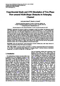
This ensures that the modified volume expansion coefficient is continuous and smooth throughout the entire region of interest. Since everything in the model for the modified volume expansion coefficient can be described as an analytical function of the mixture enthalpy, the mixture density can then be obtained

15

directly by integration using the definition in Eq. (9). The results of this model are shown in Fig. 2 as functions of the equilibrium quality compared to the real properties of water at 6 MPa [8]. For initial simulations using the HEM formulation of multiphase flow, a simplified turbulence model was used. In most RANS-type turbulence models, the eddy viscosity is calculated based on the transport of independent turbulence quantities such as turbulent kinetic energy. As a preliminary step, a simplified turbulence model is used in which the eddy viscosity and eddy conductivity are estimated using a constant turbulence multiplier 𝜇𝑡 = (𝐶𝑡 − 1)𝜇𝑚 𝜇𝑡 𝑃𝑟𝑡

(16)

𝜆

= (𝐶𝑡 − 1) 𝑐 𝑚 , 𝑝,𝑚

where an appropriate value for the turbulence multiplier is determined from parametric testing. x 10-6 15

1000

b [kg/J]

r [kg/m3]

real modeled

real modeled

800

600

400

10

5

200

0 -0.5

0

0.5

xeq

1

1.5

0 -0.5

2

0

0.5

(a)

1.5

2

(b)

real modeled

real modeled

15

b [kg/J]

758

r [kg/m3]

1

x 10-6 20

759

757

756

755 -0.15

xeq

10

5

-0.1

-0.05

0

xeq

0.05

0.1

0.15 x 10-3

(c)

0 -0.15

-0.1

-0.05

0

xeq (d)

0.05

0.1

0.15 x 10-3

Fig. 2. Mixture property models showing (a) density and (b) modified volume expansion coefficient across the complete model range and (c) density and (d) modified volume expansion coefficient across a narrow range centered at the liquid-to-two-phase transition.

16

3.

COMPUTATIONAL MODELS

Computational models were independently developed using appropriate pre-processing methodology and closure model selection strategy for each code. Sensitivity studies were completed as a first step toward full solution verification under the ANSI/ASME V&V 20 guidelines [10]. 3.1

STAR-CCM+

In the development of the STAR-CCM+ model, the potential impacts of several modelling decisions were investigated as part of a sensitivity study. Simulations of multiphase flows are always challenging because local variations in geometry and boundary conditions can have substantial impact on flow structures. This is especially true in the helical coil, where the low angle of inclination encourages separation of the two phases which is further accelerated by the persistence of the classical Dean vortex structure. Boiling closure models are almost universally developed for vertical pipes and channels, so their applicability to inclined pipe flows is not well known, and their applicability to helical coil flows is virtually untested. In the absence of detailed velocity, temperature or vapor distribution data from relevant experiments for validation of the closure models, a sensitivity assessment was used to determine which parameters may require further study. 3.2

COMPUTATIONAL MESH DEVELOPMENT

In the development of CFD models, the development of a good quality computational mesh is considered the most critical step. The computational mesh must not only accurately describe the flow geometry, but it also must appropriately discretize the volume for both the closure models and solvers to be applied. In the development of the helical coil model, two different meshing strategies were evaluated. First, the baseline STAR-CCM+ meshing process was used to develop a mesh consisting of a volumetrically filled polyhedral core with a polygonal prismatic extrusion layer extending to the surface. Second, a block structured hexahedral mesh was developed using the directed meshing features of the commercial meshing package ANSYS ICEM CFD [11]. Sensitivities of the STAR-CCM+ finite volume solution to the mesh structure were investigated for single phase water flow through the helical coil with a total mass flux of 520 kg/m2s. Walls were assumed to be non-slip with minimal surface roughness. Heat transfer was not considered, and adiabatic conditions were assumed. Coolant properties are consistent with water at the 50 K subcooling assumed for the helical coil boiling assessment. A mesh with very dense prismatic extrusion layers near the wall, shown in Fig. 3, was developed to provide a reference solution for turbulent flow in the helical coil pipe. The low Reynolds number formulation of the realizable  RANS turbulence model, which is integrated all the way to the wall rather than relying on a simplified wall function, was used in this reference case. The model name is somewhat misleading because it can be applied to turbulent flows of any Reynolds number, but it also offers limited capability to predict low Reynolds number transitions to turbulence. The model requires that sufficient resolution be included in the computational mesh to resolve the effects of the boundary layer, with values of the y+ parameter, the dimensionless boundary layer thickness, less than unity. The y+ parameter is a function of the thickness of the first cell and local flow conditions. The maximum y+ value for the mesh shown in Fig. 3 is 0.8335, the minimum is 0.3142, and the average is 0.5257. The predicted velocity profile in the cross section of the helical pipe is shown in Fig. 4. The line integral convolution is shown to highlight the secondary flow pattern, which is a classical Dean vortex structure. The predicted differential pressure using the outlet as the reference is shown in Fig. 5.

17

Fig. 3. Cross sectional distribution of computational mesh with well resolved boundary layer.

Fig. 4. Predicted velocity profile in the reference simulation using the low Reynolds number variant of the realizable k-epsilon turbulence model. Secondary flow structure is highlighted by the line integral convolution.

18

Fig. 5. Predicted differential pressure distribution in the reference simulation using the low Reynolds number variant of the realizable k-epsilon turbulence model.

While the simulation using the low Reynolds number model provides a good reference solution for the single-phase liquid flow case, it is not compatible with the Eulerian-Eulerian formulation, and the highly resolved boundary layer mesh is not appropriate for the Eulerian-Eulerian multiphase closure models. Three alternate mesh structures that are more suitable for two-phase boiling flow simulations were used to simulate the same single phase liquid flow as the reference case. The first alternate mesh, shown in Fig. 6 (a), uses the default polyhedral meshing strategy of STAR-CCM+ with the recommended settings for the prismatic extrusion layer. The second alternate mesh, shown in Fig. 6 (b), maintains the same polyhedral core mesh but radically expands the prismatic extrusion layer in an effort to regularize the cells filling the majority of the meshed volume. The third alternate mesh, shown in Fig. 6 (c) is a blockstructured hexahedral mesh similar to the reference mesh with a much coarser representation of the near wall region. Fig. 6 (d) is the refined mesh used in the reference wall-resolved low-y+ simulations.

19

(a)

(b)

(c)

(d)

Fig. 6. Computational meshes used in mesh sensitivity study: (a) nominal polyhedral core mesh, (b) polyhedral core mesh with extended prismatic extrusion layer, (c) nominal hexahedral block-structured mesh, and (d) reference wall-refined hexahedral block-structured mesh.

Simulations were completed using each of the three coarser meshes for the same single-phase flow conditions as the reference case. These simulations use the high Reynolds number formulation of the realizable  turbulence model and the all y+ two-layer wall treatment, which is more appropriate for the coarser near-wall mesh resolution. Velocity profiles along the horizontal diameter of the pipe were extracted from simulations using all four computational meshes and are shown in Fig. 7. All three of the simulations using coarser meshes predict slightly steeper velocity gradients across the pipe diameter, but the polyhedral mesh with the extended prismatic layer is the most extreme. All three also consistently predict slightly lower pressure drops in the helical coil steam generator tube. Results from the standard STAR-CCM+ polyhedral mesh and the standard block-structured hexahedral mesh are very similar. The results from the standard polyhedral mesh appear to show a slight discontinuity at the interface between the polyhedral core mesh and the prismatic extrusion layer. However, this is actually an artifact of the interpolation scheme used to extract the monitoring point data. The hexahedral mesh does provide a slight advantage in simulation convergence rate, and for this reason, the standard block-structured hexahedral mesh structure has been selected for use in the two-phase flow simulations. 20

1 Low y+ Standard Polyhedral Extended Prismatic Layer Standard Hex Mesh

0.9

Velocity Magnitude

0.8 0.7 0.6 0.5 0.4 0.3 0.2 0.1 0 0

0.1

0.2

0.3 0.4 0.5 0.6 0.7 Normalized Position Across Tube

0.8

0.9

1

Fig. 7. Predicted velocity profiles along the horizontal tube diameter for 3 alternate computational mesh configurations and the reference low y+ simulation. Data are extracted in the cross section located 1½ revolutions of the helical pipe from the inlet.

The applicability of the selected high Reynolds number variant of the realizable  turbulence model and all y+ two-layer wall treatment can be confirmed by comparing the values of the y+ parameter for the selected hexahedral mesh shown in Fig. 6 (c) with the model’s acceptable range. For the selected mesh and conditions, the maximum value of the y+ parameter is 35.98, the minimum is 15.5, and the average is 26.00. All are within the limits established for the model in the STAR-CCM+ user guide. Since the single-phase flow is quite turbulent with a Reynolds number based on the tube diameter of just over 100,000, the flow should be fully developed well before it has completed the first ½ revolution of the helix. This can be confirmed by comparing velocity profiles from positions nearer the outlet. In Fig. 8, profiles are shown from simulations using the selected block-structured hexahedral mesh with data taken from cross section planes at the first ½ revolution and at 1½ revolutions. The predicted single-phase velocity profile from simulations using the selected block-structured hexahedral mesh is shown in Fig. 9, with secondary flows highlighted by the line integral convolution. The dean vortex structure is similar to the higher resolution reference solution. The predicted pressure drop from simulations using the selected baseline hexahedral mesh is shown in Fig. 10. The predicted pressure drop is approximately 3% lower than the reference low y+ model solution.

21

0.9 1 pi

3 pi

0.8

Velocity Magnitude

0.7 0.6 0.5 0.4 0.3 0.2 0.1 0 0

0.1

0.2

0.3 0.4 0.5 0.6 0.7 Normalized Position Across Tube

0.8

0.9

1

Fig. 8. Evolution of predicted velocity profiles along the horizontal pipe diameter as coolant moves through the helix.

Fig. 9. Predicted velocity profile in the reference simulation using the high Reynolds number variant of the realizable k-epsilon turbulence model. Secondary flow structure is highlighted by the line integral convolution.

22

Fig. 10. Predicted differential pressure distribution in the reference simulation using the high Reynolds number variant of the realizable k-epsilon turbulence model.

3.3

BENCHMARKING SINGLE PHASE STAR-CCM+ PREDICTIONS

For fully developed single-phase turbulent flow in a helical coil, correlations from prediction of pressure drop have been proposed by Santini [2], Ito [12] and Ruffel [13] in the standard engineering friction factor form. The Santini model for the friction factor is based on data collected in the identified experiment at SIET. The Santini friction factor model is given as 𝑓 = 0.00206 + 0.085𝑅𝑒 −0.278,

(17)

the Ito friction factor model is give as

𝐷 −0.5

𝑓 = 0.076𝑅𝑒 −0.25 + 0.00725 ( 𝑑 )

and the Ruffel friction factor model is given as

23

,

(18)

𝐷 −0.275

𝑓 = 0.00375 + 0.633 ( 𝑑 )

Re−0.4 .

(19)

Predictions of pressure drop from single-phase simulations using the baseline mesh structure are compared with the predictions of these correlations in Fig. 11. Simulation predictions are similar to those from the correlations at equivalent conditions.

Fig. 11. Comparison of CFD predictions of single-phase pressure drop with three experimental correlations.

3.3.1

Nek5000

As an initial point of comparison, the block structured hexahedral mesh selected for use in STAR-CCM+ was also used in Nek5000. This is shown as the “initial mesh” in Fig. 12. This mesh was used for the laminar flow simulation as it is currently the only direct comparison available between Nek5000 and StarCCM+. Later meshes used in Nek5000 were generated with preNek, the native mesh generation tool developed along with Nek5000. The switch to using preNek was made because geometry information relating to curved element edges is not preserved in the conversion from the Star-CCM+ format to the Nek5000 format. This can be seen in Fig. 12, as the circular shape of the cross section in the initial mesh is only preserved to the element edges rather than to the Gauss-Lobatto-Legendre (GLL) points, as is the case with the preNek mesh. Additionally, the process of converting the mesh results in randomly ordered elements in Nek5000, whereas a preNek generated mesh will have some known element ordering structure which can be used to enhance post-processing and simplify output of averaged quantities as the simulation is in progress.

24

A third mesh was also used with Nek5000, as shown in Fig. 13. This mesh was also generated using preNek, but it made use of a scripting interface which reduced the mesh generation time from hours to seconds. The third mesh was generated because the first two did not sufficiently resolve the near-wall region. The only two-equation turbulence model available in Nek5000 is a low Reynolds number (low-y+) model, whereas Star-CCM+ includes high Reynolds number turbulence models. The third mesh also takes better advantage of the spectral nature of Nek5000. This mesh was generated using approximately 1/20th the number of elements compared to the original preNek generated mesh. However, better resolution is achieved by running at a higher spectral order, significantly increasing the accuracy of the simulation. The necessary near-wall resolution was determined using 2D axisymmetric simulations. After significant parametric testing, it was shown that a y+ value of less than 1 for the GLL point next to the wall (not on the wall) is necessary for the turbulence model. This is consistent with expectations from implementations of similar models in other CFD codes. In all turbulent 3D simulations with Nek5000, the maximum, minimum, and average next to wall y+ values were monitored as the simulation was in progress to ensure consistency.

Initial mesh

preNek mesh

Fig. 12. Cross section views of the meshes used in the initial Nek5000 simulations of the helical coil showing the initial mesh generated with STAR-CCM+ and the mesh generated using preNek. Images show both element boundaries and Gauss-Lobatto-Legendre points associated with the higher order spectral solution.

25

Turbulent mesh

Near-wall details

Fig. 13 The mesh generated for use with the κ-ω model in Nek5000 showing the cross section view and the mesh refinement close to the wall.

26

4.

LAMINAR SINGLE PHASE FLOW SIMULATIONS

To demonstrate that the underlying flow physics between the two codes are consistent, initial comparisons between Nek5000 and STAR-CCM+ simulations focused on a scenario which does not rely on the advanced modeling capabilities of either code, i.e. the turbulence model or the multiphase flow model closures. The expected heating and mass flow rates for the chosen helical coil steam generator tube were applied to the full geometry and run as a strictly single-phase flow with no turbulence model. This is not an accurate representation of the physical behavior of the tube, but it is a useful check for the consistency of the underlying Navier-Stokes solutions. 4.1

NEK5000 SIMULATIONS

A simulation was performed in Nek5000 at prototypic conditions defined in Table 2, which is a mass flux of 800 kg/m2-s, constant wall heat flux of 150 kW/m2, an inlet subcooling of -50 K, and fluid properties evaluated for water at 6MPa in a geometry corresponding to two full rotations of the helical coil. This corresponds to a Reynolds number based on the pipe diameter of just over 100,000. No turbulence or multiphase models were used. Results for two different cross sections of the helical pipe are shown in Fig. 14 and Fig. 15. These demonstrate that the flow reaches a fully developed state.

(a) Velocity [m/s]

(b) Transverse Velocity [m/s]

(c) Subcooling [oC]

Fig. 14. Cross sectional slices at ½ rotation from the inlet for the laminar, single phase Nek5000 simulation showing (a) the axial velocity with overlaid transverse vectors, (b) the transverse velocity magnitude, and (c) the subcooling. The center of the helix is on the right in all three images.

27

(a) Velocity [m/s]

(b) Transverse Velocity [m/s]

(c) Subcooling [oC]

Fig. 15. Cross sectional slices at 1 full rotation from the inlet for the laminar, single phase Nek5000 simulation showing (a) the axial velocity with overlaid transverse vectors, (b) the transverse velocity magnitude, and (c) the subcooling. The center of the helix is on the right in all three images.

The development of Dean Vortices can be seen in the transverse velocity vectors, although they are highly distorted from what is typically observed. This distortion is likely a result of the low effective viscosity. 4.2

STAR-CCM+ SIMULATIONS

As in Nek5000 simulations shown above, simulations of the prototypic conditions defined in Table 2 in the first two rotations of the helical coil. No turbulence or multiphase models were activated in these simulations. As with the Nek5000 simulations, these results are non-physical and serve only as a basis for benchmarking the underlying solution of the Navier Stokes equations. Results from the cross section after the fluid has completed one full revolution within the helical coil are shown in Fig. 16.

(a) Velocity [m/s]

(b) Transverse Velocity [m/s]

(c) Subcooling [oC]

Fig. 16. Cross sectional slices at 1 full rotation from the inlet for the laminar, single phase STAR-CCM+ simulation showing (a) the axial velocity with overlaid transverse vectors, (b) the transverse velocity magnitude, and (c) the subcooling. The center of the helix is on the right in all three images.

28

4.3

NEK5000 VS. STAR-CCM+ BENCHMARKING

In general, the two codes show good agreement for the artificially laminarized case. The codes show the development of similar secondary flow structures that resemble Dean vortices but are significantly distorted by the artificially reduced effective viscosity. The simulations show similar axial and transverse velocity magnitudes as well. The most significant differences are found in the prediction of temperature distributions. The Nek5000 predictions tend to be significantly more diffusive while STAR-CCM+ shows stronger advection of thermal energy into the flow field by the secondary flow. These differences are further explored in the evaluations of two-phase flow predictions.

29

5.

TURBULENT MULTIPHASE FLOW SIMULATIONS

While benchmarking of laminar single phase flow predictions is a useful exercise to understand differences in solver performance, the end application ultimately requires evaluation of turbulent multiphase flows inside the helical coil tube. Multiphase simulations have been completed using two separate methodologies: the multiphase mixture model capabilities of Nek5000, and Eulerian-Eulerian dispersed multiphase modeling capabilities of STAR-CCM+. 5.1

MULTIPHASE MIXTURE MODEL SIMULATIONS

A number of simulations have been performed using the homogeneous equilibrium model described in Section 2.2 combined with a simplified eddy viscosity turbulence model, as well as the more sophisticated 𝜅-𝜔 model. Turbulence is expected to play a significant role in the overall characteristics of the multiphase flow. These initial simulations were intended as a method of testing the behavior of the HEM formulation in isolation from the effects of the turbulence model. More recently, the 𝜅-𝜔 model was implemented as part of the multi-phase formulation of Nek5000 and applied to a simulation of multiphase mixture flow in a section of the helical coil heat exchanger. 5.1.1

Simplified Turbulence Model in Nek5000

In initial simulations using a simplified turbulence model, a single coefficient is used to account for the contributions of the eddy viscosity. Since detailed experimental data are not available to calibrate this simple model, the effect of the turbulence multiplier was parametrically tested. Results are presented for simulations using multiplier values of 60 and 120 in Fig. 17 as cross sectional slices of the helical domain at 1¼ rotations of the helical coil from the inlet and in at 1½ rotations of the helical coil from the inlet in Fig. 18. Changing the turbulence multiplier had only minor effects on the flow. The overall flow structures are quite similar, particularly the velocity and subcooling distributions. The volume fraction is observed to stratify somewhat more readily with the lower turbulence multiplier. However, the downstream profiles in Fig. 18 show that this stratification is short-lived in both cases as the vapor becomes well-distributed throughout the cross section by 1½ rotations. It also appears increasing the turbulence multiplier inhibits the effect of buoyancy. In the case with the lower turbulence multiplier, the peak vapor volume fraction is shifted closer to the top of the channel at 1¼ rotations compared to the case with the higher turbulence multiplier. Farther downstream the effect is diminished, as the vapor has become well distributed, decreasing the density difference which drives buoyancy.

30

𝐶𝑡 = 60 𝐶𝑡 = 120 Velocity [m/s]

Transverse velocity [m/s]

Subcooling [K]

Vapor volume fraction

𝐶𝑡 = 120

𝐶𝑡 = 60

Fig. 17. Cross sectional slices at 1¼ rotations from the inlet for the simplified turbulence model with the HEM formulation showing the axial mixture velocity overlaid with transverse velocity vectors, the magnitude of the transverse velocity, the mixture subcooling, and the vapor phase volume fraction. Each row shows results from a simulation using the identified turbulence multiplier.

Velocity [m/s]

Transverse velocity [m/s]

Vapor volume fraction

Fig. 18. Cross sectional slices at 1½ rotations from the inlet for the simplified turbulence model with the HEM formulation showing the axial mixture velocity overlaid with transverse velocity vectors and the vapor phase volume fraction. Each row shows results from a simulation using the identified turbulence multiplier.

31

5.1.2

The Regularized 𝜿-𝝎 Model in Nek5000

In addition to the constant turbulence multiplier approach, a more sophisticated turbulence model has been used. A regularized formulation of the 𝜅-𝜔 model was recently implemented in Nek5000, and a simulation combining it with the HEM formulation has been run for a section of the helical coil. The simulated domain with the 𝜅-𝜔 model corresponds the pipe section beginning one full rotation from the inlet in the previous simulations and encompasses ½ of a rotation. This is effectively the domain between 1 and 1½ rotations. This simulation is the first time that the HEM and 𝜅-𝜔 formulations have been combined. Results for the ½ rotation domain are shown in Fig. 19 and Fig. 20. The axial mixture velocity with overlaid transverse velocity vectors, the mixture subcooling, and the vapor phase volume fraction are shown in Fig. 19 at the equivalent location of 1¼ rotations whereas the turbulent quantities are shown in Fig. 20. The results in Fig. 19 can be directly compared to the simplified turbulence model results shown in Fig. 17. The results with the 𝜅-𝜔 model are most similar to the results with a turbulence multiplier of 60. However, the 𝜅-𝜔 results show significantly more flow stratification, a stronger effect due to buoyancy, and significantly different velocity distribution.

Velocity [m/s]

Transverse velocity [m/s]

Subcooling [K]

Vapor volume fraction

Fig. 19. Cross sectional slices at 1¼ rotations from the inlet for the 𝜿-𝝎 turbulence model with the HEM formulation showing the axial mixture velocity overlaid with transverse velocity vectors, the mixture subcooling, and the vapor phase volume fraction.

Turbulent kinetic energy [m2/s2]

Turbulence dissipation frequency [1/s] (log scale)

Eddy viscosity ratio

Fig. 20. Cross sectional slices at 1¼ rotations from the inlet for the 𝜿-𝝎 turbulence model with the HEM formulation showing the turbulent kinetic energy, the turbulence dissipation frequency (𝝎), and the ratio of eddy viscosity to laminar viscosity.

32

Notably, the peak axial velocity in the κ-ω results occurs at the top of the channel, compared to near the side of the channel on the inside curve of the helix. Nothing similar to this was observed with the constant turbulence multiplier. This seems to arise as an effect of buoyancy as the vapor phase is strongly concentrated in this region. In the κ-ω result, the eddy viscosity is zero very close to the wall. This can be seen in Fig. 20. This low effective viscosity likely allows the less dense vapor to rise to the top of the channel more easily compared to the constant turbulence multiplier case. This can be seen in the profile of transverse velocity magnitude in Fig. 19, where the location of maximum velocity is close to the heated wall. Additionally, the magnitude of the stratification is much more significant in the κ-ω result showing a maximum of 96% vapor compared to 61% with a constant turbulence multiplier of 60, but the distribution itself is quite similar. From these results, it is reasonable to conclude the simplified turbulence model can be used to obtain some qualitative description of the flow, but it fails to capture some of the important details necessary for a quantitative analysis. Continued efforts should be focused on using the 𝜅-𝜔 model. 5.2

EULERIAN-EULERIAN SIMULATIONS

To define a preferred methodology for analyses to be completed in the remainder of the NEAMS SGFIV HIP project, a series of studies has been completed using the Eulerian-Eulerian modeling framework described in Section 2.1 to identify appropriate closure models for the multiphase helical coil steam generator application and to evaluate sensitivity of the selected combination of models to boundary conditions. Sensitivities are evaluated against a baseline simulation using unmodified closure models as implemented in the commercial release of STAR-CCM+. 5.2.1

Baseline Multi-Phase Closure Models

In addition to the bubble/droplet dynamics force models identified in equation (4), closure models must be defined to define basic geometry of the dispersed phase, as well as the heated surface characteristics. Key models used in the baseline simulation are discussed in the following sections. 5.2.1.1

Interaction Length Scale or Bubble Diameter

The interaction length scale defines the characteristic dimension of the dispersed phase and is used as input to many other closure models. The baseline simulation and all Eulerian-Eulerian simulations presented in this report use the Kurul-Podowski model [16], implemented in the code as

𝑙𝑐𝑑 =

𝐷𝑚𝑖𝑛 (∆𝑇𝐷,𝑚𝑎𝑥 − ∆𝑇) + 𝐷𝑚𝑎𝑥 (∆𝑇 − ∆𝑇𝐷,𝑚𝑖𝑛 ) . ∆𝑇𝐷,𝑚𝑎𝑥 − ∆𝑇𝐷,𝑚𝑖𝑛

(20)

The model is typically fit to measured data relevant to the problem analyzed. Default values of the minimum and maximum bubble diameter, D min and Dmax, are 0.15 mm and 2.0 mm, respectively. The liquid subcooling that corresponds to the minimum diameter, ∆𝑇𝐷,𝑚𝑖𝑛, is 13.5 K, and the liquid subcooling that corresponds to the maximum diameter, ∆𝑇𝐷,𝑚𝑎𝑥 , is -5.0 K. In this equation, ∆𝑇 is the local subcooling.

33

5.2.1.2

Interfacial Area Density, Breakup and Coalescence

The S-gamma model [17, 18, 19] is a transport model for the moments of the diameter size distribution, including the particle number density, the interfacial area density and the volume fraction. The model can support prediction of interaction length scales, but is better suited for applications with limited phase change due to wall boiling. The Kurul and Podowski model can be expected to provide better results under the conditions in the steam generator tube. The interfacial area density, breakup, and coalescence components of the model are used in these simulations. 5.2.1.3

Drag

The drag force is a resistance force acting in the opposite direction as the motion of the bubble or particle relative to the carrier phase. The drag force on the carrier phase i due to phase j is given by 𝐷 𝐅𝑖𝑗 = 𝐴𝐷𝑖𝑗 (𝐯𝐣 − 𝐯𝐢 ),

(21)

where 𝐴𝐷𝑖𝑗 is the linearized drag coefficient. For flows with a continuous phase carrying a disperse phase, the coefficient can be written in a more typical engineering form given by 𝑎

1

𝐴𝐷𝑖𝑗 = 𝐶𝐷 2 𝜌𝑐 |𝐯𝐣 − 𝐯𝐢 | ( 4𝑖𝑗),

(22)

where 𝑎𝑖𝑗 is the interfacial area density. The baseline model considered in this study uses the drag coefficient model for pure fluids developed by Tomiyama [20], which is implemented as

𝐶𝐷 = max [min (

5.2.1.4

24 72 8𝐸𝑜 (1 + 0.25𝑅𝑒 0.687 ), ) , ]. 𝑅𝑒 𝑅𝑒 3(𝐸𝑜 + 4)

(23)

Lift

The lift force acts on particles perpendicular to the relative velocity as a consequence of velocity gradients in the carrier phase. It can be described by 𝐅𝐿 = 𝐶𝐿 𝛼𝜌𝑐 [𝐯𝑟 ×(∇×𝐯𝑐 )]

(24)

The lift coefficient can be calculated based on local bubble characteristics using the model proposed by Tomiyama [21]. The implementation in STAR-CCM+ is given by 0.288 tanh(0.121 max[𝑅𝑒, 7.374]) 𝐶𝐿 = {0.00105𝐸𝑜𝑑3 − 0.0159𝐸𝑜𝑑2 − 0.0204𝐸𝑜𝑑 + 0.474 −0.27

34

𝐸𝑜𝑑 < 4 4 ≤ 𝐸𝑜𝑑 ≤ 10. 10 < 𝐸𝑜𝑑

(25)

5.2.1.5

Turbulent Dispersion

The turbulent dispersion force accounts for the redistribution of the dispersed phase as a consequence of turbulence. It can be defined by carrying forward the Reynolds averaging process to include the instantaneous drag force. It is implemented in STAR-CCM+ in the form a drag correction given by 𝐅𝑇𝐷 = 𝐴𝐷𝑖𝑗 𝐯𝑻𝑫 ,

(26)

where the void drift velocity is defined as 𝐯𝑻𝑫 = 𝐃𝑻𝑫 𝒊𝒋 ∙ {∇ ln(𝛼𝑗 ) − ∇ ln(𝛼𝑖 )},

(27)

and the tensor diffusivity coefficient is defined as 𝜈𝑡

𝑐 𝐃𝑻𝑫 𝒊𝒋 = 𝜎 𝐈. 𝛼

(28)

The turbulent Prandtl number for void fraction is modeled using the Tchen turbulent dispersion coefficient model [22]. 5.2.1.6

Virtual Mass

The virtual mass force accounts for the influence of the inertia of the surrounding fluid on the acceleration of the particle or bubble [23]. Models are based on the difference of the acceleration vectors for the two phases and the force can be described by 𝐅𝑖𝑗𝑉𝑀 = 𝐶𝑖𝑗𝑉𝑀 𝜌𝑖 𝛼𝑗 [𝐚𝑗 − 𝐚𝑖 ].

(29)

The coefficient is modeled using the spherical particle method. 5.2.1.7

Baseline Model Results

The multiphase flow through the steam generator was simulated using the baseline closure models with fixed mass flow rate and uniform heat flux boundary conditions as specified in Table 2. As shown in Fig. 21, the steam water mixture is fully saturated by the time it completes the second rotation around the helix (4 in the polar coordinate notation used in the figure). As shown in Fig. 22, the liquid and vapor phases very quickly stratify as vapor forms in the system. Vapor first concentrates along the surface of the pipe facing the center of the helix and then rises to the upper surface. As the vapor concentrates in the upper part of the pipe, the Dean vortex structure begins to tilt, as shown in Fig. 21. The stratification is a significant feature of the helical coil steam generator tube that must be addressed in design considerations since the heat transfer may be significantly reduced in the stratified vapor layer.

35

0.5



1.5

2

2.5

3

3.5

4

Fig. 21. Evolution of temperature profile in the helical coil steam generator tube using the baseline model configuration. The center of the helix is on the right in all images. A polar coordinate notation is used to indicate position in the helix, with 2indicating one full rotation around the helix.

0.5



1.5

2.5

2

3

3.5

4

Fig. 22. Evolution of vapor distribution in the helical coil steam generator tube using the baseline model configuration. The center of the helix is on the right in all images. A polar coordinate notation is used to indicate position in the helix, with 2indicating one full rotation around the helix.

36

(a) Single-phase flow

(b) Two-phase flow

Fig. 23. Secondary flow field in the helical coil steam generator tube after 1¼ revolutions (2½ in the polar coordinate notation) around the helix for both single and two-phase flow. The center of the helix is on the right in all images.

5.2.2

Sensitivity to Closure Models

In general, multiphase boiling simulations in vertical channels exhibit extreme sensitivity to the lift coefficient, which moves large bubbles to the center of the channel and small bubbles toward the wall. However, in this case, the two phases quickly separate which limits the impact of the lift coefficient. In this case, the drag coefficient was expected to have a more significant impact on the flow field. The average value of the drag coefficient in the baseline model was estimated and constant values of the drag coefficient representing roughly one half of that value (CD = 0.2) or roughly two times that value (CD = 0.8) were used in subsequent simulations to evaluate sensitivity. As shown in Fig. 24, the change in drag coefficient has minimal impact on the predicted flow structure. Smaller coefficients encourage sharper resolution of boundaries between the two phases, and larger coefficients do result in prediction of less separation as should be expected. However, the two phases continue to clearly separate with similar interface positions in all three cases. Sensitivity to virtual mass and turbulent dispersion were not considered, but they do contribute to the stability of the simulation and converged solutions cannot be readily obtained if they are not activated.

37

Tomiyama

Cdrag = 0.8

Sauter Mean Diameter

Void Fraction

Temperature

Axial Velocity

Cdrag = 0.2

Fig. 24. Comparison of baseline simulation results (Tomiyama model) with two alternate drag coefficient models in the cross section after the flow has completed 1½ rotations (3 in polar coordinate system notation). Predicted axial velocity of the liquid phase with transverse flow structures are shown, highlighted with the line integral convolution, predicted temperature distribution, predicted void distribution and predicted Sauter mean bubble diameter.

38

5.2.3

Sensitivity to wall heat boundary conditions

In order to evaluate the sensitivity of the model to the choice of boundary conditions, an alternate model was simulated using the baseline modeling strategy with a constant wall temperature condition equivalent to a wall superheat of 4 K. For comparison, a constant heat flux case with equivalent energy addition, approximately 600 W/m2 was simulated. The predicted vapor fraction distribution from the constant wall superheat and constant heat flux cases are shown in Fig. 25. Although void profiles appear to develop somewhat more quickly in the constant wall temperature case, both cases show very similar evolutions the stratified multiphase flow.

Const. q”

Const. Tw

More significant differences can be found in the deeper details of the simulations. The Sauter mean bubble diameter is a measure of the mean bubble size in a particular computational cell. The comparison of results from constant wall temperature and constant wall temperature simulations shown in Fig. 26 indicates that the constant heat flux case predicts the a much stronger concentrations of large bubbles near the center of the pipe in the lower cross sections. However, as the fluid reaches saturation and a more clearly stratified vapor layer is established differences become less significant.

2

2.5

3

3.5

4

Fig. 25. Predicted void fractions in two comparable cases with constant wall temperature (top row) and constant wall heat flux (bottom row). The center of the helix is to the right in all images. A polar coordinate notation is used to indicate position in the helix, with 2indicating one full rotation around the helix.

39

Const. Tw Const. q”

2

2.5

3

3.5

4

Fig. 26. Predicted Sauter mean bubble diameter in two comparable cases with constant wall temperature (top row) and constant wall heat flux (bottom row). The center of the helix is to the right in all images. A polar coordinate notation is used to indicate position in the helix, with 2indicating one full rotation around the helix.

5.2.4

Sensitivity to flow rate

The nominal case defined in Table 2 is only one potential operating condition in the actual steam generator. In order to assess the applicability of the model to alternate operating scenarios, two additional cases were considered. In the first, the mass flux was reduced by half to G = 400 kg/m2s. In the second, the mass flux was increased by a factor of 1.5 to G = 1200 kg/m2s. In both cases the power-to-flow ratio was maintained. As expected, flows with lower mass fluxes show stronger rotation of the interface due to the curvature of the pipe. Additionally, the dual vortex structure of the classical Dean instability is more persistent in the high flow case. By the time the flow has made 1½ turns around the helix, the upper vortex has already collapsed in the two cases with lower flow rates. Although power–to-flow ratios were matched so that total temperature rise in the steam generator tube would be comparable across all three cases, this is not sufficient to provide similitude between the temperature distribution or Sauter mean bubble diameter. This is noted because the distribution of these parameters must be considered if scaled facilities are to be used to evaluate vibration source terms resulting from boiling and multiphase transport.

40

G=800kg/m2s

G=1200kg/m2s

Sauter Mean Diameter

Void Fraction

Temperature

Axial Velocity

G=400kg/m2s

Fig. 27. Comparison of baseline simulation results with two alternate boundary condition sets in the cross section after the flow has completed 1½ rotations (3 in polar coordinate system notation). Differences in flow rate are noted; power-to-flow ratios were maintained. Shown are predicted axial velocity with transverse flow structures highlighted with the line integral convolution, predicted temperature distribution, predicted void distribution and predicted Sauter mean bubble diameter.

41

5.3

TWO-PHASE BOILING FLOW BENCHMARKING

Most two-phase boiling pressure drop correlations follow the form of the proven Lockhart and Martinelli [24] type correlations, using a two-phase multiplier as shown below: (

𝑑𝑃 𝑑𝑃 ) = Φ𝑙2 ( ) , 𝑑𝐿 2𝜙 𝑑𝐿 𝑙

(30)

where Φ𝑙 , the only-liquid friction multiplier, has the form Φ𝑙2 =

𝑓2𝜙 𝜌𝑙 1 . (1 𝑓𝑙 𝜌𝑚 − 𝑥)2

(31)

A variant uses the liquid-only multiplier, which relates the two-phase mixture pressure drop to the singlephase pressure drop at the same mass flux as the mixture: 𝑑𝑃 2 𝑑𝑃 ) = Φ𝑙𝑜 ( ) 𝑑𝐿 2𝜙 𝑑𝐿 𝑙𝑜

(32)

2 Φ𝑙𝑜 = Φ𝑙2 (1 − 𝑥)1.8 .

(33)

(

Zhao [25] proposed a correlation for the liquid-only multiplier based on accumulated data that take the form 𝜌𝑙 2 0.282 Φ𝑙𝑜 = 1 + ( − 1) [0.303𝑥1.63 (1 − 𝑥)0.885 𝑅𝑒𝑙𝑜 + 𝑥 2 ]. 𝜌𝑔

(34)

Colombo integrated the Zhao dataset with additional data from the experiments completed in the SIET facility and proposed a correlation for the liquid-only two phase friction multiplier in the form 2 𝐷𝑒 0.19 ( Φ𝑙2 = 0.0986 Φ𝐿𝑀 𝑙

𝜌𝑚 −0.4 ) , 𝜌𝑙

(35)

2 is the only-liquid multiplier of Lockhart and Martinelli. where Φ𝐿𝑀

Simulation results over a range of exit qualities have been compared with these two correlations in Fig. 1. The Colombo correlation is reported to agree with the experimental data with 12.9% mean absolute percentage error. Predicted values from CFD are generally within this error band, but additional data should be generated for comparison near the exit quality values of 0.4, where a substantial deviation is observed.

42

Fig. 28. Comparison of predicted two-phase pressure drops from CFD simulations and two correlations.

5.4

NEK5000 VS. STAR-CCM+ COMPARISONS

Simulations of turbulent multiphase boiling flow in a helical coil steam generator tube have been completed using both the Nek5000 dispersed phase mixture model and with the STAR-CCM+ EulerianEulerian two-fluid model. Predicted void fraction distributions from these simulations are shown in Fig. 29. The two methods predict similar stratification of the gas and liquid phases, although the interface between the phases is less clearly defined in the Nek5000 mixture model simulations. Comparisons of other parameters also show similar features. This provides some confidence in the application of the Eulerian-Eulerian two-fluid method to this analysis.

(a) Nek5000

(b) STAR-CCM+

Fig. 29. Comparison of predicted void fraction distributions after the fluid has moved through 1¼ rotations of the helical coil from Nek5000 mixture model (left) and STAR-CCM+ Eulerian-Eulerian two-fluid simulations (right).

43

6.

FUTURE WORK

The work discussed in this report demonstrates that CFD-based capabilities can be applied to assessments of vapor generation and flow features in helical coil steam generator tubes. However, these studies also highlight the importance of key experimental data that simply do not exist, namely detailed measurements of void, temperature, and velocity distributions in the cross section of the tube. In order to fill this critical validation data gap, an air-water experiment that can provide these detailed measurements will be pursued in the next year of the project, in addition to continued CFD analyses. Upcoming CFD simulation efforts will leverage two recent development efforts related to the Nek5000 and STAR-CCM+ codes to improve both uncertainty assessments and benchmarking. A two-phase twofluid capability called Nek-2P [26] has been implemented within Nek5000 to provide a high-order Eulerian-Eulerian dispersed phase simulation capability, which will serve as a benchmark for further STAR-CCM+ simulations. Additionally, STAR-CCM+ has been integrated with the Dakota toolset for sensitivity and uncertainty quantification analysis [27]. Dakota will be used to drive more extensive sensitivity assessments for the final application of the demonstrated simulation capability.

44

7.

CONCLUSIONS

The NEAMS steam generator flow induced vibration (SGFIV) high impact problem (HIP) team was established to demonstrate the applicability of tools developed by the NEAMS program to the identification and mitigation of vibration sources in advanced steam generator designs, such as helical coil steam generators. Three sub-teams were established to analyze transient turbulent flow structures as the primary coolant flows over the outside of the steam generator tubes, to analyze the multi-phase boiling characteristics of the secondary flow inside the tubes, and to integrate information from those two simulations into a finite element method structural mechanics analysis of the tubes and their support structure. This report summarizes the demonstration of a methodology for the multiphase boiling flow analysis inside the helical coil steam generator tube. A helical coil steam generator configuration is defined based on the experiments completed by Polytecnico di Milano in the SIET helical coil steam generator tube facility. Simulations of the defined problem were completed using the Eulerian-Eulerian multi-fluid modeling capabilities of the commercial CFD code STAR-CCM+. Simulations suggest that the two phases will quickly stratify in the slightly inclined pipe of the helical coil steam generator. These results have been successfully benchmarked against both empirical correlations for pressure drop and simulations using an alternate CFD methodology, the dispersed phase mixture modeling capabilities of the open source CFD code Nek5000.

45

REFERENCES 1. J. Amicis, A. Cammi, L.P.M. Colombo, M. Colombo, and M. E. Ricotti, “Experimental and numerical study of the laminar flow in helically coiled pipes,” Progress in Nuclear Energy 76 (2014) 206–215. 2. L. Santini, A. Cioncolini, C. Lombardi, and M. Ricotti, “Two-phase pressure drops in a helically coiled steam generator,” International Journal of Heat and Mass Transfer 51 (2008) 4926–4939. 3. SIET S.p.A., homepage, http://www.siet.it (2016). 4. STAR-CCM+, version 11.02.010, (2015). 5. E. Baglietto, and M. A. Christon, “Demonstration and Assessment of Advanced Modeling Capabilities for Multiphase Flow with Sub-cooled Boiling,” CASL-U-2013-0181-001 (2013). 6. A. Tomboulides, S. M. Aithal, P. M. Fischer, E. Merzari, and A. Obabko, “A novel variant of the K-𝜔 URANS model for spectral element methods – implementation, verification and validation in NEK5000,” in Proc. of ASME (2015). 7. A. Tentner, P. Vegendla, A. Obabko, A. Tomboulides, P. Fischer, O. Marin, and E. Merzari, “Modeling of two-phase flow in a BWR fuel assembly with a highly-scalable CFD code,” in Proc. Of NURETH-16 (2016). 8. S. A. Klein, Engineering Equation Solver. Madison, Wisconsin: F-Chart Software, 2015. 9. T. Yabuki and O. Nakabeppu, “Microscale wall heat transfer and bubble growth in single bubble subcooled boiling of water,” Int. J. Heat and Mass Transfer, 100 (2016) 851–860. 10. 2008 ANSI Standard V&V 20. ASME Guide on Verification and Validation in Computational Fluid Dynamics and Heat Transfer, 2009. 11. ANSYS ICEM CFD, version 16.0, 2015. 12. H. Ito, “Friction factors for turbulent flow in curved pipes,” J. Basic Eng. (1959) 123–134. 13. A. E. Ruffell, “The application of heat transfer and pressure drop data to the design of helical coil once-through boilers,” Symp. Multi-Phase Flow Systems, University of Strathclyde, Inst. Chem. Eng. Symp. Ser. 38 (1974), Paper 15. 


14. Y. Cengiz, B. Yasar, B., and P. Dursun, “Heat transfer and pressure drops in rotating helical pipes,” ApplEnergy, 50 (1995) 85–94. 
 15. L. Guo, X. Chen, C.Z. Feng, C.Z., and B. Bai, “Transient convective heat transfer in a helical coiled tube with pulsatile fully developed turbulent flow,” Int J Heat Mass Transfer 41 (1998) 2867–75.

16. N. Kurul and M. Podowski, “Multidimensional effects in sub-cooled boiling”, Proceedings of the Ninth Heat Transfer Conference, Jerusalem (1990). 17. S. Lo and P. Rao, “Modelling of droplet breakup and coalescence in an oil-water pipeline,” 6th Int. Conf. Multiphase Flow, ICMF 2007, Leipzig, Germany (2007). 
 18. S. Lo, and A. Tomasello, “Recent progress in CFD modelling of multiphase flow in horizontal and near-horizontal pipes,,” 7th North America Multiphase Technology, Banff, Canada (2010). 
 19. S. Lo, and D/ Zhang, “Modelling of Break-up and Coalescence in Bubbly Two-Phase Flows,” J. Comp. Multiphase Flows, 1 (2009) 23-–38. 


46

20. A. Tomiyama, I. Kataoka, I. Zun, , and T. Sakaguchi, “Drag Coefficients of single bubbles under normal and micro gravity conditions,” JSME International Journal, Series B, 41 (1998) 472–479. 21. A. Tomiyama, H. Tamai, I. Zun, I., and S. Hosokawa, “Transverse migration of single bubbles in simple shear flows,” Chemical Engineering Science, 57 (2002) 1849–1858. 
 22. D. Thai-Van, J. P. Minier, O. Simonin, P. Freydier , and J. Olive, “Multidimensional two-fluid model computation of turbulent dispersed two-phase flows,” ASME FED, 185 (1994) 277–291. 
 23. T. R. Auton, J. C. R. Hunt, and M. Prud’homme, “The force exerted on a body in inviscid unsteady non-uniform rotational flow,” J. Fluid Mech., 197 (1988) 241–257. 
 24. R. W. Lockhart and R. C. Martinelli, “Proposed Correlation of Data for Isothermal Two Phase Flow, Two Component Flow in Pipes,” Chem. Eng. Prog., 45 (1949) 39–48.

25. L. Zhao, L. Guo, B. Bai, Y. Hou, and X. Zhang, “Convective boiling heat transfer and two-phase flow characteristics inside a small horizontal helically coiled tubing once through steam generator,” Int. J. Heat Mass Transfer, 46 (2003) 4779–4788. 26. A. M. Tentner, P. Vegendla, A. Tomboulides, A. Obabko, E. Merzari, and D. Shaver, Advances in the development of Nek-2p: a two-phase flow modeling capability for the Nek5000 CFD code,” Proceedings of CFD4NRS-6, Cambridge, MA, USA (2016). 27. M. -O. Delchini, E. Popov, W. D. Pointer, and L. P. Swiler, L. P., Assessment of SFR Wire Wrap Simulation Uncertainties, Oak Ridge National Laboratory, ORNL/TM-2016/540 (2016).

47