Evaluation of Cluster Identification Performance for ... - Semantic Scholar

Volume 29 (2010), Number 3

Eurographics/IEEE-VGTC Symposium on Visualization 2010 G. Melançon, T. Munzner, and D. Weiskopf (Guest Editors)

Evaluation of Cluster Identification Performance for Different PCP Variants Danny Holten1 and Jarke J. van Wijk1 1 Eindhoven

University of Technology, The Netherlands

Abstract Parallel coordinate plots (PCPs) are a well-known visualization technique for viewing multivariate data. In the past, various visual modifications to PCPs have been proposed to facilitate tasks such as correlation and cluster identification, to reduce visual clutter, and to increase their information throughput. Most modifications pertain to the use of color and opacity, smooth curves, or the use of animation. Although many of these seem valid improvements, only few user studies have been performed to investigate this, especially with respect to cluster identification. We performed a user study to evaluate cluster identification performance – with respect to response time and correctness – of nine PCP variations, including standard PCPs. To generate the variations, we focused on covering existing techniques as well as possible while keeping testing feasible. This was done by adapting and merging techniques, which led to the following novel variations. The first is an effective way of embedding scatter plots into PCPs. The second is a technique for highlighting fuzzy clusters based on neighborhood density. The third is a spline-based drawing technique to reduce ambiguity. The last is a pair of animation schemes for PCP rotation. We present an overview of the tested PCP variations and the results of our study. The most important result is that a fair number of the seemingly valid improvements, with the exception of scatter plots embedded into PCPs, do not result in significant performance gains. Categories and Subject Descriptors (according to ACM CCS): I.3.3 [Computer Graphics]: Picture/Image Generation—Line and Curve Generation I.3.3 [Computer Graphics]: Picture/Image Generation—Viewing Algorithms H.5.2 [Information Interfaces and Presentation]: User Interfaces—Evaluation/Methodology

1 Introduction Information visualization techniques that are able to effectively and efficiently depict multivariate (multidimensional) data can provide valuable insight when analyzing such data. Two examples of recurring tasks that are commonly performed when analyzing multivariate data are the identification of correlation between data variables and the identification of clusters of data points. Parallel coordinate plots (PCPs) [Ins85, ID90] are a wellknown visualization technique for depicting and analyzing multivariate data. PCPs visualize multivariate data by displaying k parallel axes representing the data variables (coordinates). Each k-dimensional data point is mapped to a polyline with vertices on these parallel axes. The position of a vertex on the i-th axis corresponds to the i-th coordinate of a data point. The aforementioned correlation and cluster identification are two classes of tasks that are effectively supported by PCPs [AA01]. Although various alternative multivariate visualization techniques [Che73, Cle85, War94, HGM∗ 97] as well as 3D adaptations of PCPs [FCI05, SEO∗ 06] exist, 2D PCPs are c 2010 The Author(s)

c 2010 The Eurographics Association and Blackwell Publishing Ltd. Journal compilation Published by Blackwell Publishing, 9600 Garsington Road, Oxford OX4 2DQ, UK and 350 Main Street, Malden, MA 02148, USA.

still one of the most popular techniques for visualizing multivariate data. An advantage of PCPs is that they provide a continuous and comparative view across parallel axes (data variables) as well as a comparative view across polylines (data points). This facilitates identification of correlation and clusters, respectively. However, a disadvantage when visualizing large amounts of data is that PCPs tend to suffer from visual clutter resulting from intersections and overlapping polylines, which may obscure important patterns. As a result, various visual modifications to PCPs were introduced to facilitate tasks such as correlation and cluster identification, to reduce visual clutter, and to increase the general information throughput of PCPs. As described in Section 2, most of these modifications pertain to the use of color and opacity, smooth or bundled curves, or animation. Although many of these modifications seem valid improvements, only few user studies have been performed that formally evaluated the effectiveness of PCPs, something which is also noted by Li et al. [LMvW08]. The studies that we know of furthermore focus on correlation identification, not on cluster identification [JLJC06, FJ07, JFLC08,

Danny Holten & Jarke J. van Wijk / Evaluation of Cluster Identification Performance for Different PCP Variants

LMvW08]. Finally, Kosara et al. [KHI∗ 03] note that visualization as currently practiced is mostly a craft and evaluation is often performed informally. The use of user studies should therefore be encouraged. This is also noted by North [Nor06], who states that there are too many informal usability studies that only indicate whether participants liked a certain visualization technique. We therefore evaluated PCP-based cluster identification performance, the second important class of PCP-supported tasks as identified by Andrienko et al. [AA01]. To our knowledge, no user studies have been performed that focus on cluster identification performance using PCPs. Li et al. [LMvW08] furthermore acknowledge the importance of evaluating PCP-based cluster identification performance next to their evaluation of correlation identification performance using either scatter plots or PCPs. We analyzed cluster identification performance of nine PCP variations, including standard PCPs. In short, each participant was asked to perform a number of cluster identification trials for each PCP variation. For each trial they had to answer how many clusters were being displayed. We generated various stimuli for this that contained between two and six clusters. Response times and correctness were measured and analyzed using one-way ANOVA and Tukey’s HSD (Honestly Significant Difference) post-hoc test to determine whether or not there were significant performance differences between the nine PCP variations. To generate the PCP variations, we focused on covering existing techniques that provide visual modifications to PCPs as well as possible while keeping testing feasible. This was done by adapting and merging existing techniques into nine final PCP variations, which additionally contain various novel elements. The first novel addition is an effective way of embedding scatter plots into PCPs. The second is a technique for highlighting fuzzy clusters using color and opacity based on the neighborhood density of each data point. The third is a spline-based alternative to polylines to reduce certain forms of ambiguity. Finally, the last comprises a pair of animation schemes for PCP-based rotations of multivariate data points. These are introduced to augment PCPs with motion cues such as parallax that could ease cluster detection. The remainder of this paper is organized as follows. Section 2 presents related work on PCPs: alternatives, user studies, and visual modifications. Section 3 provides an overview of the tested variations and describes our novel additions. Section 4 and 5 describe the design and results of our user study, respectively. Finally, Section 6 presents our conclusion and recommendations for future work. 2 Related Work Since we aim at covering existing techniques as well as possible with our tested PCP variations, we first provide a thorough overview of various PCP-specific modifications such as color- and opacity-based cluster enhancement, the use of smooth and bundled curves instead of polylines, and anima-

tion. PCP-related user studies and alternative multivariate visualization techniques are also discussed. 2.1 Cluster Enhancement This section describes various color- and opacity-based cluster enhancement techniques for PCPs that could facilitate cluster identification. Hierarchical Parallel Coordinates (HPCs) [FWR99] provide an interactive, multiresolution data view via hierarchical clustering. Artero et al. [AdOL04] propose a way to emphasize patterns in PCPs by calculating frequency and density information from a data set to control an opacitybased rendering method that depicts PCPs as filtered frequency and density plots. Johansson et al. [JLJC06] emphasize clusters in PCPs by using a high-precision texture to store a basic PCP to which a transfer function (TF) is applied to obtain the final color- and opacity-based rendering. An outlier-preserving visualization technique for PCPs is presented in [NH06] which treats precomputed outliers and clusters separately during visualization. Visual clustering (VC) in PCPs as introduced by Zhou et al. [ZYQ∗ 08] applies color based on local line density. Color is assigned through user-defined TFs. Lastly, an animated splatting framework for cluster detection in PCPs is presented in [ZCQ∗ 09]. At each animation step, a polyline is splatted into the PCP and neighboring polylines are either enhanced or suppressed. Many of these methods rely on explicit cluster computation [FWR99, JLJC06, ZCQ∗ 09] or require interaction to highlight or extract clusters [FWR99, AdOL04, NH06, ZYQ∗ 08, ZCQ∗ 09]. We choose to focus on basic, noninteractive PCP variations. User interaction would significantly complicate testing and since even basic variations have not been previously evaluated with respect to cluster identification performance, we argue that these should be tested first. We furthermore contend that if cues such as color, opacity, curves, or animation can lead to a significant advantage when applied to standard PCPs, this should already be noticeable when testing basic variations. We also refrain from explicit computation of (a user-specified number of) clusters, since this could introduce misleading information on the actual number of clusters in the data, because a discrete number of clusters is being forced on the data. Instead, we present a new highlighting method for fuzzy clusters using color and opacity based on the local neighborhood density of each data point (Section 3.2). Our method does not require user intervention and also works on fuzzy clusters, without requiring explicit cluster computation. 2.2 Smooth and Bundled Curves Since it might be easier to visually follow smooth curves than polylines, Smooth PCPs [MW02] were introduced to replace polylines with curves that cross PCP axes orthogonally. Curves are also used by Graham & Kennedy [GK03] and Yuan et al. [YGX∗ 09] to allow data points to be traced under certain limitations (Fig. 3a and b) without requiring

c 2010 The Author(s)

c 2010 The Eurographics Association and Blackwell Publishing Ltd. Journal compilation

Danny Holten & Jarke J. van Wijk / Evaluation of Cluster Identification Performance for Different PCP Variants

curves to cross PCP axes orthogonally (Fig. 3c). This reduces unnecessary curvature. We provide a simple splinebased drawing method akin to [GK03,YGX∗ 09] that furthermore enables one to control the amount of smoothing, providing a continuous trade-off between polyline- and curvebased PCPs (Section 3.3). Illustrative Parallel Coordinates (IPC) [MM08] and the VC approach by Zhou et al. [ZYQ∗ 08] furthermore employ curves to generate edge-bundled PCPs. IPC relies on the availability of explicit clusters while VC generates varying numbers of visually distinct clusters depending on the settings used. Both methods are therefore less suited for the enhancement of fuzzy clusters. 2.3 Animation As described by Ellis & Dix [ED07], augmenting information visualization techniques with animation can facilitate visual clutter reduction and keep users oriented. This is also noted by Heer & Robertson [HR07], who show how user orientation can be preserved using animated transitions between visualization states. There a relatively few examples of PCP-specific animation techniques [JLJC06]. Stuart et al. [SWB02] and Barlow & Stuart [BS04] show how animation can be applied to PCPs to enhance the understanding of time-varying data variables. Feature animation is furthermore used by Johansson et al. [JLJC06] to convey statistical properties about clusters present in PCPs. Finally, Wegman & Luo [WL96] show how PCPs can be interactively explored using Grand Tours [Asi85], a method for viewing multivariate data via projections of rotated multidimensional data points onto 2D subspaces. In Section 3.4, we introduce a pair of animation schemes inspired by Grand Tours to augment PCPs with parallax motion cues that could facilitate cluster detection. 2.4 User Studies User studies comparing PCPs to other techniques are the comparative study of Stardinates and PCPs by Lanzenberger et al. [LMP05] and a study on multivariate visualization techniques by Pillat et al. [PVF05]. Johansson et al. and Forsell & Johansson [FJ07] have conducted various user studies on the identification of correlation between data variables in 2D and 3D PCPs [JLJC06, FJ07, JFLC08]. Li et al. [LMvW08] have also focused on correlation in their user study. They evaluated the analysis of correlation using both 2D scatter plots and 2D PCPs. 2.5 Alternative Multivariate Visualizations Although the focus of this paper is on the specific assessment of cluster identification performance of visual modifications to 2D PCPs, the following lists alternative multivariate visualization techniques that also support the identification of correlation and clusters. Chernoff Faces [Che73] show multivariate data by using individual elements of the human face to represent data val-

c 2010 The Author(s)

c 2010 The Eurographics Association and Blackwell Publishing Ltd. Journal compilation

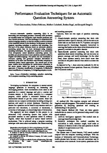
ues. The popular scatter plots technique [Cle85] uses 2D/3D Cartesian coordinate systems to display 2D/3D data points. For data sets of higher dimensionality, scatter plot matrices [SS05,WAG05] show all of the pairwise 2D scatter plots in the form of a matrix. XmdvTool [War94] incorporates a multivariate visualization technique known as a radar plot, Kiviat diagram, star plot, or Stardinates. It employs a radial chart with k axes representing the k data variables on top of which k-dimensional data points are shown as k-sided polygons. Using force-directed placement, Radviz [HGM∗ 97] positions k-dimensional data points within a k-sided polygon, the corners of which represent the k data variables. Various 3D extensions to PCPs exist as well. Examples are 3D Parallel Coordinate Systems [SEO∗ 06] and the 3D integration of PCPs and star plots [FCI05]. 3 Parallel Coordinate Plot Variations This section contains a description of the tested PCP variations. As mentioned in Section 1, we aimed at covering existing techniques as well as possible while keeping testing feasible. This led to nine basic, non-interactive PCP variations that were tested. These variations additionally contain four novel elements presented in the following subsections. To prevent excessively dark regions due to overdraw while retaining outlier visibility, our base case (first PCP variation) is a standard 2D PCP using black polylines at 25% opacity on a white background (Fig. 4a). This constant value was chosen after initial trials in which similar stimuli were used as during the actual user study (Section 4.3), with opacity ranging from 5% to 100% in 5% increments. We contend that since constant blending has practically become a standard feature of the majority of modern, practical PCP implementations, our base case – using constant blending, a high-resolution display, and anti-aliasing – is quite representative of modern, minimalistic PCP representations. Furthermore, constant blending as used in the base case still differs significantly from the more advanced blending mode as described in Section 3.2, which is actually put forward as an additional PCP variation. An OpenGL-based Windows application written in Borland Delphi 7 was used to display all of the visualizations at 16x anti-aliasing. 3.1 Scatter Plots Embedded into PCPs Although we focus on PCPs, one of the most well-known multivariate visualization techniques for 2D data are scatter plots. Instead of showing a k×k scatter plot matrix for kdimensional data to provide a 2D scatter plot for each data variable combination, we embed 2D scatter plots between each pair of adjacent PCP axes. This saves screen space and still provides a 2D scatter plot for each pair of adjacent axes as defined by the PCP axes ordering. Axis labels are furthermore shared effectively by rotating the scatter plots 45◦ . The embedding is shown in Fig. 1 and scatter plots embedded into PCPs are used as the second PCP variation (Fig. 4b).

Danny Holten & Jarke J. van Wijk / Evaluation of Cluster Identification Performance for Different PCP Variants

Figure 1: Scatter plots embedded into a PCP. Red arrows denote the direction of the a1 axis in each visualization. 3.2 Enhancement of Fuzzy Clusters As explained in Section 2.1, we refrain from computing explicit clusters because of the possible introduction of misleading information due to a discrete number of clusters being forced on the data. We furthermore want to be able to emphasize fuzzy clusters as well. We therefore introduce a color- and opacity-based highlighting method for fuzzy clusters using the local neighborhood density of each data point. Let n ≥ 2 be the number of data points in a k-dimensional data set. The average distance di of a data point pi , 0 ≤ i < n, to its neighbor points is defined as dr(n−2)e

di = r Ni

: :

1 dr(n−2)e+1

·

∑

|pi − Ni [ j]|,

j=0

neighborhood range, 0 < r ≤ 1; distance-sorted neighbor points of pi .

to facilitate cluster discrimination, not show order. We are furthermore aware that density-based coloring will not assign (fully) unique colors to fuzzy clusters in case of similar densities. However, the majority of our stimuli showed a fair number of clearly distinct colors. Although our synthetic stimuli contain explicit clusters, we also want our method to apply to data that does not contain explicit clustering information. In the special case of explicit clusters, a discrete palette containing a fixed number of easily distinguishable colors, e.g., as provided by ColorBrewer [HB03], would be better suited. PCPs using density-based coloring are used as the third PCP variation (Fig. 4c). It is furthermore possible to control polyline opacity using the amount of enhancement by having ei = 0 and ei = 1 map to a minimum and maximum opacity multiplication factor, respectively. We settled on 0.25 and 1 for our visualizations. PCPs using density-based blending are used as the fourth PCP variation (Fig. 4d). Finally, it is straightforward to combine density-based coloring and blending, resulting in the fifth PCP variation (Fig. 4e). Figure 2: The color LUT used for density-based coloring running from low (left) to high (right) cluster density. 3.3 Curves instead of PCP Polylines As shown in Fig. 3, ambiguity caused by polyline crossing is not resolved by curves that cross PCP axes orthogonally [MW02]. To ease visual tracking of data points across data variables, we introduce a curve drawing method that resolves crossing ambiguity by only introducing curvature where needed as shown in Fig. 3d.

The neighborhood range r determines the number of closest neighbor points of pi that are used to calculate di . Neighbors of pi are stored in Ni and are sorted from closest to most distant using a k-dimensional Euclidean distance measure. The minimum and maximum values of di in a data set are used to compute the normalized distance kdi k, 0 ≤ kdi k ≤ 1. The amount of enhancement ei , 0 ≤ ei ≤ 1, of a data point pi can now be defined as ei = 1 − kdi k. Small values of r result in more localized enhancement (which is somewhat more susceptible to noise due to undersampling), whereas large values result in more globalized (smoother) enhancement. We settled on r = 13 for our visualizations, which suppresses most of the noise while retaining fairly strong localized enhancement. The enhancement is used as follows to control color- and opacity-based rendering of PCP polylines. A polyline corresponding to a point pi is colored using a lookup table (LUT) as shown in Fig. 2. ei = 0 and ei = 1 map to colors at the left and right of the color LUT, respectively. Although rainbow-like color maps are considered not ideal for encoding ordinal values, our main goal is to maximize the number of distinct, smoothly interpolated colors

Figure 3: Polyline crossing ambiguity (a,b) is not solved by (c) curves crossing PCP axes orthogonally. (d) Our approach resolves this ambiguity while minimizing curvature. For a vertex p on a polyline crossing a PCP axis, a tangent is introduced whose slope is identical to that of the line between p0 and p1 , p’s neighboring vertices. Curve smoothness s, 0 ≤ s ≤ 1, is used to adjust tangent length from 0 (resulting in standard polylines) to the distance between adjacent axes (maximum smoothness). c 2010 The Author(s)

c 2010 The Eurographics Association and Blackwell Publishing Ltd. Journal compilation

Danny Holten & Jarke J. van Wijk / Evaluation of Cluster Identification Performance for Different PCP Variants

Figure 4: The six non-animated PCP variations that were evaluated: (a) standard PCP, (b) scatter plots embedded into a PCP, (c) colored polylines, (d) blended polylines, (e) colored and blended polylines, and (f) curves instead of polylines.

Figure 5: Five frames of a random tour animation show the movement of two clusters. Initially (dotted lines), clusters exhibit considerable overlap, making it hard to distinguish them. Parallax introduced by animation helps to visually separate clusters. Since polylines cross at p0 , no unnecessary curvature is introduced. If the polylines would have “reflected” at p0 , our method would have introduced curvature to show this, thus resolving ambiguity. Curve segments between adjacent PCP axes are drawn using cubic Bézier splines, whose control points are determined by the polyline–PCP axis intersections and the tangent end points. PCPs using curves instead of polylines are used as the sixth PCP variation (Fig. 4f), employing a medium curve smoothness of s = 0.5. 3.4 Animated PCPs Another way to facilitate cluster identification is the addition of animation to PCPs. This introduces motion parallax, which helps to visually separate overlapping clusters (Fig. 5). We now describe the augmentation of PCPs with a pair of animation schemes as inspired by Grand Tours [Asi85], two of which – the random tour and the permutation tour as described in the following – were used before in a similar fashion in the specific context of PCP animation [Asi85, WL96]. First, a random permutation r of the data dimensions {0, . . . , k − 1} is generated. A pair of consecutive axes (dimensions) in r, i.e., r[i] and r[i + 1], with 0 ≤ i < k, defines a matrix Ri (t, ωi ). This time-dependent rotation matrix Ri (t, ωi ) expresses a rotation in the 2D (r[i], r[i + 1])-plane of α radians around the origin, where α = ωi · t. Ri (t, ωi ) is essentially an identity matrix that differs at four posi-

c 2010 The Author(s)

c 2010 The Eurographics Association and Blackwell Publishing Ltd. Journal compilation

tions to generate a rotation matrix, i.e., let Ri (t, ωi ) = R, then Rr[i],r[i] = cos α, Rr[i],r[i+1] = − sin α, Rr[i+1],r[i] = sin α, and Rr[i+1],r[i+1] = cos α. Each Ri is assigned a random an11 2 2π ≤ ωi ≤ 100 2π. This range gular velocity ±ωi , with 100 was chosen after initial assessment showed that it resulted in polyline clusters that move fast enough to quickly create parallax while still enabling viewers to visually track them. Sequential application of all rotation matrices Ri by means of matrix multiplication defines the final rotation matrix M(t) used to rotate all data points as k−2

M(t) =

∏ Ri (t, ωi ).

i=0

This random tour animation scheme is used as the seventh PCP variation (Fig. 5). It generates animations that are virtually non-cyclic, thus always showing new patterns. Wegman [Weg90] showed that for k-dimensional data, the minimal set P of PCP axis permutations necessary so that every possible axis adjacency occurs contains (k + k mod 2)/2 permutations. An alternative animation scheme can be constructed from this by smoothly cycling through all of these permutations, showing viewers all possible axis adjacencies in an animated fashion. This is done by encoding an axis ordering (permutation) as an orthonormal matrix Oi , 0 ≤ i < (k + k mod 2)/2. To generate the matrix Oi corresponding to permutation Pi , the non-zero elements of Oi are Oi [r, c], with 0 ≤ r < k and c = Pi [r]. A 4D example:

Danny Holten & Jarke J. van Wijk / Evaluation of Cluster Identification Performance for Different PCP Variants

Pi = {2, 0, 3, 1} ⇒

0 1 0 0

0 0 0 1

1 0 0 0

0 0 1 0

! = Oi .

The final rotation matrix M(t) used to rotate all data points is generated by first determining – by using t and the desired permutation transition speed s – which permutations are being interpolated. This gives the corresponding orthonormal matrices Oi and Oi+1 . The exact interpolation progress t 0 , 0 ≤ t 0 ≤ 1, between Oi and Oi+1 is now determined (again by using t and s) and subsequently used to define the final t0 rotation matrix as (Oi+1 · O−1 i ) · Oi . This permutation tour animation scheme is used as the eighth PCP variation. The transition speed s was chosen such that the average on-screen animation speed of the polylines matched that of the random tour scheme. We furthermore guaranteed a frame rate of 30fps+ for both schemes under all circumstances. We now introduce a third and final animation scheme for more localized animations, i.e., PCP polylines that “wobble” around a fixed base position in a sinusoidal way. This also generates helpful motion parallax, but keeps clusters fairly fixed, thus easing visual tracking. For this, we use the random tour scheme as basis and adapt M(t) by using t M 0 (t) = M(t + δ(t)) and δ(t) = a · sin( 2π), T a : wobble amplitude (seconds); T : wobble period time (seconds). a is also in seconds, since it defines the neighborhood around t = 0 in the random tour scheme that is “scanned” during a wobble cycle. We settled on a = 0.1s and T = 1s, resulting in rapid parallax while retaining the local character of the animation with respect to cluster position. The wobble animation scheme is used as the ninth PCP variation. 4 Evaluating Cluster Identification Performance This section provides information on the design of the conducted user study as well as its participants. 4.1 User Study Design We used a repeated-measures, within-subjects design with nine factors represented by the PCP variations that we wanted to evaluate. For each participant, a test comprised nine subtests – one for each variation – and each subtest comprised 16 trials (synthetic stimuli): one test and 15 real trials. This amounts to 144 trials and 135 measurements per participant. For each trial, participants identified the number of clusters, and response time and correctness were recorded. Two to six clusters were used; a maximum of six was chosen since viewers experienced great difficulties when confronted with more than six clusters in trial runs. Subtest order was randomized for each participant to compensate for possible carry-over effects such as learning or fatigue. Per subtest, each cluster count case – two to six – appeared three times in a random order (participants were not made aware of this). Each stimulus was only used once per participant and the same stimuli were presented – in random order and randomly assigned to subtests – to all participants.

4.2 Evaluation Procedure Each participant was interviewed before testing to obtain the information presented in Section 4.5. The concept of PCPs was introduced and participants were told they were going to count clusters (also called “ribbons”) using PCP variations. The variations were shortly presented and we made sure that participants understood the task. Participants were told to use the number keys on the keyboard to enter trial answers. While a trial was presented, participants pressed the space bar when they were confident about their answer to stop timing and clear the screen. They could then input their answer, after which the next trial was automatically started. Participants were instructed to determine their own pace, the important thing being that they try to behave consistently during testing. They were furthermore allowed to shortly pause (approximately one minute) between subtests to tell us how they experienced the evaluated PCP variation. 4.3 Stimulus Generation For all stimuli, the number of data dimensions was kept fixed at six. To generate a stimulus with c clusters, a cloud containing 125 to 175 (random) points with radius 1 was generated using a Gaussian distribution to represent background noise. c Gaussian clusters (radius 0.15 to 0.25, random) containing 100 to 150 (random) data points were then generated and randomly position within the background. These values are the result of preliminary testing during pilot trials. Although we are aware of the fact that the chosen number of points is fairly small when viewed in a real-world context, one of the reasons why we chose this number was to be able to guarantee smooth animations. Furthermore, user interaction, e.g., selection and filtering, is generally needed to select an interesting subset from a large data set consisting of hundreds of thousands of points. Since we chose not to test the effect of user interaction (to keep testing feasible), we refrained from very large data sets as well. The chosen settings allow for some variation while generating stimuli that contain clusters that – with moderate effort – can be clearly identified as such. We furthermore removed degenerate cases from the stimuli prior to the user study. 4.4 Test Apparatus and Setup Tests were conducted on an HP EliteBook 8530w laptop with an NVIDIA Quadro FX 770M graphics card, external keyboard, and a Dell E228WFP 22" LCD screen. Trials were shown fullscreen at 1680×1050 pixels and viewing distance was approximately 70cm. The same location was consistently used and tests were performed during the daytime under normal indoor lighting conditions (fluorescent lamps). Setup orientation was such that glare was eliminated. 4.5 Participants In total, twenty participants, twelve male and eight female, took part in our user study. Thirteen were part of faculty, scientific staff, or students. All twenty had at least a bachelor-

c 2010 The Author(s)

c 2010 The Eurographics Association and Blackwell Publishing Ltd. Journal compilation

Danny Holten & Jarke J. van Wijk / Evaluation of Cluster Identification Performance for Different PCP Variants

level education and eleven were familiar with PCPs. Ages ranged from nineteen to fifty and all participants declared to have normal or corrected-to-normal full-color vision. 5 Evaluation Results In this section, we describe our initial hypotheses and provide a discussion of the results of the conducted user study. 5.1 Hypotheses We henceforth refer to the nine PCP variations as Standard, SP (scatter plot), Color, Blend, ColorBlend, Curved, RT (random tour), PT (permutation tour), and Wobble. Color is generally regarded as a very strong visual cue and we furthermore expected positive reinforcement from multiple cues. We therefore expected ColorBlend at first place, followed by Color. Because of the intuitiveness of scatter plots, we expected SP at third place. Curved was expected next, since it might resolve ambiguities and help in following polylines across axes. Blend – put at fifth place – was expected to be a stronger cue than motion parallax because of its noise suppression. Animations were expected at places six through eight, with Wobble at sixth place due to its localized animations that might ease cluster tracking. Because of the similarities between RT and PT, we had no clear preference for either of them. Finally, we expected all variations to outperform Standard due to the presence of additional cues. In summary, the expected order was hColorBlend, Color, SP, Curved, Blend, Wobble, {RT, PT}, Standardi. 5.2 Main Results Regarding both response time and correctness, there was no significant difference between men and women, nor between participants with and without PCP experience. With respect to increasing cluster count, response time and correctness showed virtually similar kinds of increase and decrease patterns, respectively, for all of the PCP variations, clearly indicating increasing task difficulty (Fig. 6).

picts the correlation graphically. Based on this observation, we can facilitate analysis by only analyzing response time using one-way ANOVA and Tukey’s HSD test, since the results for correctness follow a similar pattern.

Figure 7: There is a strong correlation (r = −0.88) between response time and correctness. Each point represents a unique combination of PCP variation and cluster count. To evaluate if there was a significant performance difference between at least two of the nine PCP variations, we performed a one-way within-subjects ANOVA test with the nine PCP variations as independent variables and response time as the single dependent variable. For each PCP variation, response time measurements were normalized per cluster count case before being used as input for the ANOVA analysis. Fig. 8 shows the average response time for each of the tested PCP variations.

Figure 8: Average response time for each of the PCP variations (shown with a 95% confidence interval).

Figure 6: Response time and correctness plotted against cluster count show similar patterns for all PCP variations. The graphs in Fig. 6 together hint at a strong correlation between response time and correctness with respect to cluster count, which is indeed the case: the Pearson correlation r between response time and correctness is -0.88. Fig. 7 dec 2010 The Author(s)

c 2010 The Eurographics Association and Blackwell Publishing Ltd. Journal compilation

ANOVA analysis showed that there was a significant effect of PCP variation type, F(8, 2691) = 15.28, p < 0.05. Although Fig. 8 already provides some insight regarding the variations between which a significant difference probably exists, we additionally performed a post-hoc analysis for pairwise comparison using Tukey’s HSD test to further investigate the pairwise differences. Fig. 9 shows the results. As expected from Fig. 8, only SP performs significantly better than five of the remaining eight variations. RT and PT perform even significantly worse than all of the remaining PCP variations, even worse than Standard. The following section discusses these surprising findings in more detail.

Danny Holten & Jarke J. van Wijk / Evaluation of Cluster Identification Performance for Different PCP Variants

Figure 9: Tukey’s HSD test results. For α = 0.05, 9 treatments, and a within-groups df > 1000 (2691 in our case), all values > 4.39 (bold and green) show a significant difference. 5.3 Discussion We first want to mention that the results discussed in this section should be interpreted as an initial step in investigating the performance of different PCP variations. To keep testing feasible, choices had to be made with respect to which (and how many) PCP variations to evaluate, what type of task to evaluate, what class of data to use, and whether or not user interaction would be part of the testing procedure. To be able to provide a stronger statement regarding the performance of various PCP representations in general, additional user studies will have to be performed that address the limitations described above (see Section 6.1). To our surprise, our initial hypotheses regarding the expected order of PCP variations as presented in Section 5.1, i.e., hColorBlend, Color, SP, Curved, Blend, Wobble, {RT, PT}, Standardi, is largely superseded by the discovered order (based on Fig. 9): hSP, {Standard, Color, Blend, ColorBlend, Curved, Wobble}, {RT, PT}i. Only one of the PCP variations, SP, clearly outperformed Standard as expected. In addition, SP was the only variation that contained visualization elements that were non-PCPspecific, i.e., scatter plots. Nevertheless, this result was already somewhat expected before analysis, since a recurring remark made by virtually all participants was that they experienced SP as the least difficult variation. It should be noted that participants were clearly instructed to view the SPs as complementary to the PCP representation. They were also made aware of the fact that ambiguity might be present in either of the representations; they were told how the other representation could be used to clarify things in such cases. Furthermore, this result is complementary to the findings of Li et al. [LMvW08], who concluded that scatter plots are more effective than PCPs in supporting visual correlation analysis. With respect to PCP-based cluster identification, the second important class of PCP-supported tasks [AA01], we could conclude that scatter plots are more effective overall than PCPs as well. However, it should be noted that although participants were apparently able to use embedded scatter plots to perform efficient quantitative analyses, i.e., identifying the number of clusters, a PCP representation might still be better suited for certain qualitative analyses, e.g., obtaining insight in the actual shapes of the clusters. It should furthermore be noted that apart from SPs, it is

also possible to enrich PCPs with other visualization elements, e.g., histograms overlayed onto PCP axes [HLD02], to obtain quantitative as well as qualitative insight regarding clusters. SPs were mainly chosen because they are one of the most well-known multivariate visualization techniques and because we furthermore had to limit the number of PCP variations to keep testing feasible. With the exception of SP, RT, and PT, there are no significant differences between the remaining PCP variations. Especially Color(Blend) did not perform nearly as well as we expected, regardless if color is generally deemed a strong visual cue. However, this finding is still in line with the fact that SP, not Color (or any other variation for that matter), was repeatedly pointed out as the clear favorite by participants. A possible explanation might be that participants tended to forcefully ignore color, since our coloring method did not assign fully unique colors to all clusters in case of similar densities. Although the majority of the stimuli showed clearly distinct colors, participants might still have preferred to determine cluster count without relying on colors that are not fully unique, thus trying to avoid mistakes. One of the things that participants virtually unanimously agreed on was that RT and PT proved exceptionally hard due to visual tracking problems, especially if the cluster count was five or six. Again, this remark is in line with our analysis results, which show that fully animated tours are best avoided. If one wishes to add animation to PCPs, a more localized animation method is probably a better choice than fully animated tours. The exceptional difficulty of RT and PT in case of five or six clusters furthermore agrees with studies conducted by Yantis [Yan92], who showed that visually tracking more than five objects at a time is difficult. 6 Conclusion Apart from various novel additions to PCP-based visualizations, our user study on PCP-based cluster identification performance led to surprising and unexpected results as described in Section 5. Nevertheless, these findings agree with what the vast majority of participants subjectively remarked about the tested variations. In addition, our findings on fully animated tours in PCPs agree with previous studies on multielement visual tracking [Yan92] as well. Because of the fact that the obtained results are somewhat limited to the conditions of our user study (as mentioned in Section 5.3), further investigation is warranted to support the more general and far-reaching statement that the majority of visual modifications put forward to improve PCPs do not always work (too well) in practice. However, we argue that even our current findings – with respect to PCP-based cluster identification tasks, the tested PCP variations, and the class of data that comprised the stimuli – should be taken as an encouragement to not simply regard a visualization as an improvement just because it seems feasible from a visual point of view. Formal evaluations are actually needed to determine if this is the case [KHI∗ 03, Nor06].

c 2010 The Author(s)

c 2010 The Eurographics Association and Blackwell Publishing Ltd. Journal compilation

Danny Holten & Jarke J. van Wijk / Evaluation of Cluster Identification Performance for Different PCP Variants

The following section discusses some possible directions of future work to allow for more general remarks on the performance differences between PCP variations.

References

6.1 Future Work To expand the applicability of the results, additional PCP variations should be investigated. Interesting candidates include alternative animation schemes as well as cluster highlighting methods based on different concepts than neighborhood density to guide blending and coloring. Especially because of the unexpectedly poor performance of color as a visual cue and the possible explanation for this (Section 5.3), we regard additional evaluation of cluster highlighting methods that use fully unique colors, such as the ones provided by ColorBrewer [HB03], as an important follow-up investigation. Such a validation could be used to determine if color is indeed a less helpful visual cue with respect to PCP-based cluster identification, or if our results are mainly due to colors being not fully unique. To be able to do this, explicit clusters need to be calculated for each data set, which might require user guidance with respect to certain clustering parameters to reach a satisfying result. This automatically introduces the need to include user interaction as part of possible follow-up evaluations. User interaction in the form of selection and filtering should furthermore be added to follow-up user studies that make use of large data sets, another important future work direction to further generalize the results. A possible direction for additional future work is the evaluation of combinations of visual cues that might improve cluster identification in PCPs. Examples are combinations of the specific PCP variations that we tested; ColorBlend is already an example of such a combination. Various additional combinations as well as combinations comprising more than two cues could be evaluated to determine if such combinations indeed result in increased performance. This could lead to interesting outcomes such as 1) combined performance being the average of the performances of the comprising variations, 2) combined performance being increased due to positive reinforcement of multiple visual cues, or 3) combined performance being decreased due to negative interference of multiple visual cues. As a final possible direction for future work, other tasks than quantitative cluster identification could be performed, e.g., qualitative cluster analysis tasks that measure the performance of identifying clusters with certain properties using different PCP variations.

[AdOL04] A RTERO A. O., DE O LIVEIRA M. C. F., L EVKOWITZ H.: Uncovering Clusters in Crowded Parallel Coordinates Visualizations. In Proc. IEEE INFOVIS (2004), pp. 81–88. 2

7 Acknowledgements We thank all of the participants that took part in our user study. This research is part of the Expression Of Interest (EOI) project, which is supported by the VIEW programme of the Netherlands Organisation for Scientific Research (NWO) under research grant no. 643.100.502.

c 2010 The Author(s)

c 2010 The Eurographics Association and Blackwell Publishing Ltd. Journal compilation

[AA01] A NDRIENKO G., A NDRIENKO N.: Constructing Parallel Coordinates Plot for Problem Solving. In Proc. Symposium on Smart Graphics (2001), pp. 9–14. 1, 2, 8

[Asi85] A SIMOV D.: The Grand Tour: A Tool for Viewing Multidimensional Data. Journal on Scientific and Statistical Computing 6, 1 (1985), 128–143. 3, 5 [BS04] BARLOW N., S TUART L. J.: Animator: A Tool for the Animation of Parallel Coordinates. In Proc. IEEE INFOVIS (2004), pp. 725–730. 3 [Che73] C HERNOFF H.: The Use of Faces to Represent Points in k-Dimensional Space Graphically. Journal of the American Statistical Association 68, 342 (1973), 361–368. 1, 3 [Cle85] C LEVELAND W. S.: The Elements of Graphing Data. Wadsworth Publishing Company, 1985. 1, 3 [ED07] E LLIS G., D IX A.: A Taxonomy of Clutter Reduction for Information Visualisation. IEEE TVCG (Proc. INFOVIS) 13, 6 (2007), 1216–1223. 3 [FCI05] FANEA E., C ARPENDALE S. M., I SENBERG T.: An Interactive 3D Integration of Parallel Coordinates and Star Glyphs. In Proc. IEEE INFOVIS (2005), pp. 149–156. 1, 3 [FJ07] F ORSELL C., J OHANSSON J.: Task-Based Evaluation of Multi-Relational 3D and Standard 2D Parallel Coordinates. In Proc. IS&T/SPIE Electronic Imaging, Volume 6495 (2007), pp. 64950C:1–12. 1, 3 [FWR99] F UA Y.-H., WARD M. O., RUNDENSTEINER E. A.: Hierarchical Parallel Coordinates for Exploration of Large Datasets. In Proc. IEEE VIS (1999), pp. 43–50. 2 [GK03] G RAHAM M., K ENNEDY J.: Using Curves to Enhance Parallel Coordinate Visualisations. In Proc. IEEE INFOVIS (2003), pp. 10–16. 2, 3 [HB03] H ARROWER M. A., B REWER C. A.: Colorbrewer.Org: An Online Ttool for Selecting Color Schemes for Maps. The Cartographic Journal 40 (2003), 27–37. 4, 9 [HGM∗ 97] H OFFMAN P. E., G RINSTEIN G. G., M ARX K., G ROSSE I., S TANLEY E.: DNA Visual and Analytic Data Mining. In Proc. IEEE VIS (1997), pp. 437–441. 1, 3 [HLD02] H AUSER H., L EDERMANN F., D OLEISCH H.: Angular Brushing of Extended Parallel Coordinates. In Proc. of IEEE INFOVIS (2002), pp. 127–130. 8 [HR07] H EER J., ROBERTSON G.: Animated Transitions in Statistical Data Graphics. IEEE TVCG (Proc. INFOVIS) 13, 6 (2007), 1240–1247. 3 [ID90] I NSELBERG A., D IMSDALE B.: Parallel Coordinates: A Tool for Visualizing Multi-Dimensional Geometry. In Proc. IEEE VIS (1990), pp. 361–378. 1 [Ins85] I NSELBERG A.: The Plane with Parallel Coordinates. The Visual Computer 1, 4 (1985), 69–91. 1 [JFLC08] J OHANSSON J., F ORSELL C., L IND M., C OOPER M.: Perceiving Patterns in Parallel Coordinates: Determining Thresholds for Identification of Relationships. Information Visualization 7, 2 (2008), 152–162. 1, 3 [JLJC06] J OHANSSON J., L JUNG P., J ERN M., C OOPER M.: Revealing Structure in Visualizations of Dense 2D and 3D Parallel Coordinates. Information Visualization 5, 2 (2006), 125–136. 1, 2, 3

Danny Holten & Jarke J. van Wijk / Evaluation of Cluster Identification Performance for Different PCP Variants [KHI∗ 03] KOSARA R., H EALEY C. G., I NTERRANTE V., L AID LAW D. H., WARE C.: Thoughts on User Studies: Why, How, and When. IEEE CG&A 23, 4 (2003), 20–25. 2, 8 [LMP05] L ANZENBERGER M., M IKSCH S., P OHL M.: Exploring Highly Structured Data: A Comparative Study of Stardinates and Parallel Coordinates. In Proc. INFOVIS (2005), pp. 312–320. 3 [LMvW08] L I J., M ARTENS J.-B., VAN W IJK J. J.: Judging Correlation from Scatterplots and Parallel Coordinate Plots. Information Visualization (2008). 1, 2, 3, 8 [MM08] M C D ONNELL K. T., M UELLER K.: Illustrative Parallel Coordinates. Computer Graphics Forum (Proc. EUROVIS) 27, 3 (2008), 1031–1038. 3 [MW02] M OUSTAFA R. E. A., W EGMAN E. J.: On Some Generalizations of Parallel Coordinate Plots. In Seeing a Million – A Data Visualization Workshop, Rain am Lech, Germany (2002). 2, 4 [NH06] N OVOTNÝ M., H AUSER H.: Outlier-Preserving Focus+Context Visualization in Parallel Coordinates. IEEE TVCG (Proc. INFOVIS) 12, 5 (2006), 893–900. 2 [Nor06] N ORTH C.: Toward Measuring Visualization Insight. IEEE CG&A 26, 3 (2006), 6–9. 2, 8 [PVF05] P ILLAT R. M., VALIATI E. R. A., F REITAS C. M. D. S.: Experimental Study on Evaluation of Multidimensional Information Visualization Techniques. In Proc. CLIHC’05 (2005), pp. 20–30. 3 [SEO∗ 06] S TREIT M., E CKER R. C., Ö STERREICHER K., S TEINER G. E., B ISCHOF H., BANGERT C., KOPP T., ROGO JANU R.: 3D Parallel Coordinate Systems – A New Data Visualization Method in the Context of Microscopy-Based Multicolor Tissue Cytometry. Cytometry Part A 69, 7 (2006), 601–611. 1, 3 [SS05] S EO J., S HNEIDERMAN B.: A Rank-by-Feature Framework for Interactive Exploration of Multidimensional Data. Information Visualization 4, 2 (2005), 96–113. 3 [SWB02] S TUART L., WALTER M., B ORISYUK R.: Visualisation of Neurophysiological Data. In Proc. IEEE INFOVIS (2002). 3 [WAG05] W ILKINSON L., A NAND A., G ROSSMAN R.: GraphTheoretic Scagnostics. In Proc. IEEE INFOVIS (2005), pp. 157– 164. 3 [War94] WARD M. O.: XmdvTool: Integrating Multiple Methods for Visualizing Multivariate Data. In Proc. IEEE VIS (1994), pp. 326–333. 1, 3 [Weg90] W EGMAN E. J.: Hyperdimensional Data Analysis Using Parallel Coordinates. Journal of the American Statistical Association 85, 411 (1990), 664–675. 5 [WL96] W EGMAN E. J., L UO Q.: High Dimensional Clustering Using Parallel Coordinates and the Grand Tour. In Computing Science and Statistics, Symp. on the Interface (1996), pp. 361– 368. 3, 5 [Yan92] YANTIS S.: Multielement Visual Tracking: Attention and Perceptual Organization. Cognitive Psychology 24, 3 (1992), 295–340. 8 [YGX∗ 09] Y UAN X., G UO P., X IAO H., Z HOU H., Q U H.: Scattering Points in Parallel Coordinates. IEEE TVCG (Proc. INFOVIS) 15, 6 (2009), 1001–1008. 2, 3 [ZCQ∗ 09] Z HOU H., C UI W., Q U H., W U Y., Y UAN X., Z HUO W.: Splatting the Lines in Parallel Coordinates. Computer Graphics Forum (Proc. EUROVIS) 28, 3 (2009), 759–766. 2 [ZYQ∗ 08] Z HOU H., Y UAN X., Q U H., C UI W., C HEN B.: Visual Clustering in Parallel Coordinates. Computer Graphics Forum (Proc. EUROVIS) 27, 3 (2008), 1047–1054. 2, 3

c 2010 The Author(s)

c 2010 The Eurographics Association and Blackwell Publishing Ltd. Journal compilation