Evaluation of Computational Intelligence Methods ...

Mecánica Computacional Vol XXXIV, págs. 1389-1397 (artículo completo) Sebastián Giusti, Martín Pucheta y Mario Storti (Eds.) Córdoba, 8-11 Noviembre 2016

EVALUATION OF COMPUTATIONAL INTELLIGENCE METHODS USING STATISTICAL ANALYSIS TO DETECT STRUCTURAL DAMAGE Rafaelle P. Finotti, Aldemon L. Bonifácio, Flávio S. Barbosa and Alexandre A. Cury Programa de Pós-Gradução em Modelagem Computacional, Universidade Federal de Juiz de Fora, Campus Universitário - Bairro Martelos - Juiz de Fora - MG, 36.036-330, Brasil, [email protected], [email protected], [email protected], [email protected], http://www.ufjf.br/pgmc

Keywords: Structural Dynamics, Damage Identification, Computational Intelligence. Abstract. Structural damage detection using dynamic measurements has led to the development of several approaches in the last decades. Most of conventional methods associate modal variations of the structure to damage, like methods based on strain energy deviation, methods based on changes in curvature mode shapes, flexibility matrix analysis, etc. However, the technique used to extract the modal parameters can considerably affect the results of damage identification methods, introducing additional uncertainties. Thus, approaches involving computational intelligence and statistics to detect structural changes directly from raw dynamic measurements are being investigated in recent researches. The present work aims to compare several computational intelligence algorithms to identify structural damage using statistical parameters of structural time histories. The proposed algorithms are analyzed in a numerical model of a simply supported beam. The good results encourage the development of computational tools using statistical analysis for structural damage assessment.

Copyright © 2016 Asociación Argentina de Mecánica Computacional http://www.amcaonline.org.ar

1390

1

R.P. FINOTTI, A.L. BONIFACIO, F.S. BARBOSA, A.A. CURY

INTRODUCTION

Damage in structures can be caused by design flaws, constructive problems, structural overload or natural events. Structural Health Monitoring (SHM) allows damage prevention and maintenance to ensure safe conditions for users (Cachot et al., 2015). The interest in damage identification is an important topic for engineering researches and has gained increasing attention over the years. In this context, some techniques to detect and evaluate structural damage using vibration data have been discussed, as it can be seen in Alvandi & Cremona (2006) and Alves et al. (2015). SHM has as primary aim the development of reliable and robust techniques able to detect, locate and quantify the affected regions of the structure. Due to the fact that deterioration process mainly reduces structural stiffness and modifies vibrational characteristics, damage identification approaches are usually based on changes in modal parameters or in raw dynamic measurements. Considering damage assessment using modal data, several approaches were developed: The Modal Assurance Criterion (MAC), employed as a correlation indicator between damaged and undamaged mode shapes; the Strain Energy Method (SEM), indicator based on mode shapes curvature with and without damage; analysis of flexibility matrix, among others. Although the aforementioned methods are efficient in numerical models, they present some difficulties in practical applications while dealing with experimental data. Furthermore, the technique used to extract the modal parameters can considerably affect the results of damage identification methods, introducing additional uncertainties (Alvandi & Cremona, 2006). In an effort to give alternatives to these issues, approaches interpreting raw dynamic response using statistical analysis and computational intelligence for pattern recognition have been suggested, such as in Haritos & Owen (2004); Iwasaki et al. (2004); Wen et al. (2007) and Alves et al. (2015). The focus of this work is to evaluate a strategy to detect structural damage based on Higher-Order Statistics (HOS). The statistical indicators of structural time histories are used as inputs to the following computational intelligence technologies: Multiple Linear Regression, Multiple Polynomial Regression (quadratic and cubic), Artificial Neural Network, Support Vector Machine and Random Forests. The fundamental idea is that HOS allows distinguishing apparently similar databases by inferring new statistical properties from higherorder cumulants, whereas the computational methods can recognize similar observations in a database and separate them into groups that share similar characteristics. The results given by each algorithm are analyzed and compared within a numerical model of a simply supported beam. 2

STATISTIC APPLIED IN VIBRATIONAL DATA

Most of dataset are completely characterized by the first and second-order statistics i.e., the mean value and the variance, respectively. However, there are situations in which these statistics do not provide enough information, requiring further techniques to characterize the signal. Higher-Order Statistics (HOS) is a technique that uses higher-order cumulants to infer new properties from the data (De la Rosa et al., 2013). For the case of structural dynamic data, the measured signals are very similar whether in the presence of damage or not. Therefore, the HOS can provide parameters to identify subtle differences among the dynamic measurements, enabling the detection of structural modifications. The ten different statistical indicators (first, second, third and fourth order) used in this work to characterize the dynamic responses are listed in Table 1. Copyright © 2016 Asociación Argentina de Mecánica Computacional http://www.amcaonline.org.ar

Mecánica Computacional Vol XXXIV, págs. 1389-1397 (2016)

Peak (SI1): x peak  max x Mean Squared (SI3): 1 n xsq   ( xi ) 2 n i 1 Variance (SI5): 1 n  2   ( xi  x ) 2 n i 1 Skewness (SI7): 1 n ( xi  x )3  n s  i 1 4

 Crest factor (SI9): x Cf  peak rms

1391

Mean (SI2): 1 n x   xi n i 1 Root Mean Squared (SI4): 1 n rms   ( xi )2 n i 1 Standard Deviation (SI6): 1 n   ( xi  x )2 n i 1 Kurtosis (SI8): 1 n ( xi  x ) 4  n k  i 1 4



K-factor (SI10): Kf  x peak  rms

Table 1: Statistical Indicators (Farrar & Worden, 2012).

3

COMPUTATIONAL INTELLIGENCE METHODS TO DETECT DAMAGE

Computational learning methods are considered useful tools for solving structural damage assessment problems. These algorithms work as classifiers, which try to identify damage levels using, as input data, features extracted from dynamic response (Haritos & Owen, 2004; Wen et al., 2007; Alves et al., 2015). In the next paragraphs, some concepts of computational intelligence technologies used in this study are presented. 3.1 Multiple Linear Regression (MLR) and Polynomial Regression (PR) Regression analysis can be defined as statistical techniques for modeling the relationship between one dependent variable, Y, and one or several independent variables, X or (X1, X2,…, Xn) (Gujarati & Dawn, 1999). The regression that involves only one independent variable X is called simple regression. When two or more independent variables are involved is called multiple regression. In this study it was used the Multiple Linear Regression (MLR) and Polynomial Regression (PR), which is considered a special case of MLR. These regression models are described by:

yi  (0  1 xi1 

 n xin )k   i ,

(1)

where n is the number of independent variables, i is the i-th observation, yi is the value of the dependent variable, ( 0 , 1 , ,  n ) are the model coefficients, xin is the independent variable,  i is the associated error and k indicates the polynomial degree. The regression method is determined by the index k, thus:

Copyright © 2016 Asociación Argentina de Mecánica Computacional http://www.amcaonline.org.ar

1392

R.P. FINOTTI, A.L. BONIFACIO, F.S. BARBOSA, A.A. CURY

k = 1: Multiple Linear Regression (MLR); k = 2: Quadratic Polynomial Regression (PR2); k = 3: Cubic Polynomial Regression (PR3). 3.2 Artificial Neural Network (ANN) ANNs are adaptive learning machines built from many different processing elements (PE), called neurons. In pattern classification problems, the decision surface is divided into regions representing the classes. The boundary decisions are estimated in a learning process and constructed from the statistic variability among classes (Principe et al., 2000). The most common ANN is the Multilayer Perceptron (MLP), a feedforward network composed of interconnected processing elements trained with nonlinear functions. Each PE connection has two associated adjustable parameters, weight and bias, scaled by backpropagation algorithms (learning rules) in order to minimize the error between the predicted and measured output. As explained in Principe et al. (2000), the PEs sum all of these contributions and yield an output that is a nonlinear function of the result. The training stage is an iterative process that only finishes when a stopping criterion is achieved. At the end, the perceptron is able to generalize other inputs that belong to the same class, which were not used for training. 3.3 Support Vector Machine (SVM) Another popular artificial intelligence technology for pattern recognition problem is the SVM, a statistical learning algorithm trained to determine the boundary between two classes of data in a space, where an optimal separating hyperplane is constructed in order to maximize the margin and minimize the misclassification (Vapnik, 1995). The maximization of the margin is based on an optimization function to minimize the Euclidian norm of the vector that defines the direction of the separating hyperplane. The training data points located at the margins are called support vectors. For non-linear binary classification, the inputs are mapped into a high-dimensional feature space through a kernel function. The kernel Gaussian function is used in this paper, which is also called Radial Basis Function (RBF). In this case, the SVM has two free parameters that need to be specified:  from the RBF kernel function; and C, a regularization parameter from the formulation of the margin maximization, used to avoid data overfitting. These parameters are estimated by training the SVM for multiple values of C and  . Then, the pair that minimizes the generalization error is chosen. 3.4 Random Forests (RF) Random Forest is a computational intelligence algorithm for classification and regression problems, where the idea is to build multiple decision tress based on a method called Bagging. According Breiman (2001), Bagging is a sampling technique to create multiple classification models with randomly selected subsamples of the training data, in order to use them to get an aggregated classifier (global model). Thus, each tree does a classification for a given input and the RF model returns as output the class which have the most votes (Breiman, 2001).

Copyright © 2016 Asociación Argentina de Mecánica Computacional http://www.amcaonline.org.ar

Mecánica Computacional Vol XXXIV, págs. 1389-1397 (2016)

4

1393

NUMERICAL TEST

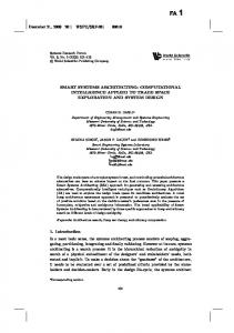
4.1 Description of the beam model The present section analyzes the proposed approach through a numerical application using a finite element model of a 6m simply supported beam (Alves et al., 2015). The mechanical properties of the beam are: Young’s Modulus (E) = 210 GPa Density = 7850 kg.m-3 Cross-Section Area = 2.81 x 10-3 m² Moment of Inertia = 2.845 x 10-8 m4 The finite element model consists of 200 elements with two nodes and two degrees-offreedom each (vertical translation and rotation). This beam is excited by a random force during 1s with different frequencies and amplitudes, applied at 0.69m from the right support, as it can be seen in Figure 1. The dynamic responses are considered as vertical accelerations measured at ten equidistant points (channels) of the beam during 100s, with a sampling rate of 100Hz, simulating an actual instrumentation made by means of accelerometers.

Figure 1: Simply supported beam model.

Three different levels of damage are simulated: Undamaged – Class 1: healthy beam; Damage level 1 – Class 2: 20% reduction of Young’s modulus at the midspan of the beam, represented by the gray color in Figure 1; Damage level 2 – Class 3: 10% reduction of Young’s modulus at the quarter length of the beam, represented by the black color in Figure 1, plus damage level 1. Furthermore, three levels of noise are added to the measurements in each structural configuration aforementioned: noiseless; 5% signal/noise (noise 1) and 10% signal/noise (noise 2). The corresponding noise levels are simulated as shown in Eq. (2):

xi ,noise  xi  nnoise . Xi .V

N (0,1) ,

(2)

where xi ,noise is the noisy signal vector, x i is the noiseless signal vector, nnoise is the noise level,  Xi is the standard deviation and V

N (0,1) is a Gaussian vector with zero mean and

unit standard deviation. Ten different dynamic tests are simulated for each level of damage and each level of noise, totaling 900 signals (10 tests x 10 channels x 3 damage levels x 3 noisy level = 900). A typical response obtained for one of these tests is shown in Figure 2. Copyright © 2016 Asociación Argentina de Mecánica Computacional http://www.amcaonline.org.ar

1394

R.P. FINOTTI, A.L. BONIFACIO, F.S. BARBOSA, A.A. CURY

Figure 2: Typical response of the beam model.

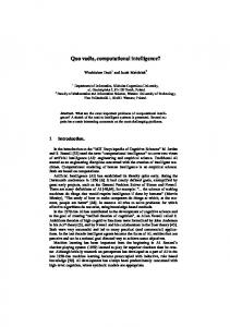
In the present application, the input dataset is arranged in a matrix [900x11] where the rows are the samples (the dynamic tests), the first ten columns are the statistical indicators and the last column indicates the position associated to the simulated accelerometer where the respective response was measured (from 1 to 10). For the ANN algorithm, the output data classes are represented by a target matrix [900x3], where the rows indicate the sample category through the binary encoding: (1 0 0) – No damage; (0 1 0) – Damage level 1 and, (0 0 1) – Damage level 2. However, for the other algorithms, the three damage classes of the input data are represented by a target vector encoded as: 1 – No damage; 2 – Damage 1 and, 3 – Damage 2. The models created from computational intelligence methods in this study, as well as the statistics indicators, were developed using toolboxes and built-in functions available in R software (MLR, PR2, PR3, SVM, RF) and Matlab (ANN). The implemented neural network is a MLP with 20 neurons in the hidden layer. The MLP was trained performing the 10-fold cross-validation method (Kohavi, 1995). LevenbergMarquadt optimization method (Hagan & Menhaj, 1994) was chosen as training function, using the mean square to assess the error and a sigmoid hyperbolic tangent as activation function. Figure 3 shows an example of the network architecture for the proposed ANN model. The SVM algorithm was trained using Gaussian Radial Basis Function kernel, where the best parameters  = 0.794328 and C = 100 were selected by training the SVM for different values of these parameters in a 10-fold cross-validation. The multi-class classification problem was solved by using one-against-one strategy (Bishop, 2006). For the Random Forest method, two values were previously specified: Ntree = 500 and mtry = 3, that indicate the number of trees and the number of input parameters used in each decision tree, respectively.

Copyright © 2016 Asociación Argentina de Mecánica Computacional http://www.amcaonline.org.ar

1395

Mecánica Computacional Vol XXXIV, págs. 1389-1397 (2016)

Figure 3: MLP network architecture with 20 neurons in the hidden layer (B1 and B2 are the bias term).

5

RESULTS

The results of the computational intelligence models are presented in Table 2. All algorithms proposed in this study were executed 30 times with 10-fold cross-validation and the classification rate is represented by the mean values of these 30 repetitions. The results are the percentages of the correct classifications for the respective damage levels of each case (number of correct classifications divided by the number of executions). Method

Mean

MLR PR2 PR3 ANN SVM Random Forest

45.79% 58.49% 67.53% 83.92% 92.20% 91.54%

Standard Deviation 5.00% 4.68% 5.00% 1.57% 2.75% 2.82%

Max.

Min.

58.89% 71.11% 82.22% 86.30% 98.89% 97.78%

27.78% 45.56% 55.56% 79.90% 83.33% 82.22%

Table 2: Correct classification rate achieved for the simply supported numerical beam.

Table 2 shows that the values obtained by PR2 and PR3 were better than MLR. Therefore, one can conclude that there is nonlinearity between input and output data, what reinforces the choice of ANN, SVM and RF for the present damage detection problem, once these algorithms achieved good classification rates.

Copyright © 2016 Asociación Argentina de Mecánica Computacional http://www.amcaonline.org.ar

1396

6

R.P. FINOTTI, A.L. BONIFACIO, F.S. BARBOSA, A.A. CURY

DISCUSSIONS AND CONCLUSIONS

In this work, a strategy to detect structural damage based on Higher-Order Statistics (HOS) and computational intelligence technologies was evaluated. The statistical parameters of structural time domain measurements were used as input for the following computational methods: Multiple Linear Regression (MLR), Multiple Polynomial Regression (quadratic – PR2 and cubic – PR3), Artificial Neural Network (ANN), Support Vector Machine (SVM) and Random Forests (RF). The proposed approach was investigated by comparing the classification results of each mentioned computational intelligence method, through a numerical model of simply supported beam. To simulate the practical feasibility of this approach, three levels of noise were added to the signals. By analyzing the performance of MLR, PR2 and PR3, it was observed the nonlinearity between input and output data, once the correct classification rates increased from 49.79% (MRL) to 58.49% (PR2), and from 58.49% (PR2) to 67.53% (PR3). The ANN, SVM and RF obtained good results for the present damage classification problem. However, SVM and RF had similar performances and allowed better classification rates than ANN, achieving results around 92%. The average classification performances show that statistical indicators in addition to computational intelligence methods were efficient in detect structural damage for the numerical beam model, where the HOS and the other statistical parameters provided sufficient information to identify subtle differences among the dynamic signals, enabling the detection of structural changes. The main advantage of using the damage prediction method presented here is to deal with data coming directly from the structure, without the need to transform them into the frequency domain to extract structural features. These previous observations encourage the development of computational tools using statistical analysis for damage assessment. Nevertheless, more investigation is required to validate this damage identification strategy, such as checking the algorithms for experimental data and for other structures. Once the computational intelligence methods were evaluated, this strategy may include weights for each parameter of input data, focusing on the best performance of the damage identification process, in order to reduce the input parameters and computational complexity. 7

ACKNOWLEDGEMENTS

The authors would like to thank UFJF (Universidade Federal de Juiz de Fora - Programa de Pós-Graduação em Modelagem Computacional), CAPES (Coordenação de Aperfeiçoamento de Pessoal de Nível Superior), CNPq (Conselho Nacional de Desenvolvimento Científico e Tecnológico - "National Council of Technological and Scientific Development") and FAPEMIG (Fundação de Amparo à Pesquisa do Estado de Minas Gerais) for the financial support. REFERENCES Alvandi, A., Cremona, C., Assessment of vibration-based damage identification techniques. Journal of Sound and Vibration, 292(1):179-202, 2006. Alves, V., Cury, A., Roitman, N., Magluta, C., Cremona, C., Structural modification assessment using supervised learning methods applied to vibration data. Engineering Structures, 99:439-448, 2015. Bishop, C.M., Pattern recognition and machine learning. Springer-Verlag, 2006. Breiman, L., Random forests. Machine learning, 45(1):5-32, 2001. Copyright © 2016 Asociación Argentina de Mecánica Computacional http://www.amcaonline.org.ar

Mecánica Computacional Vol XXXIV, págs. 1389-1397 (2016)

1397

Cachot, E., Vayssade, T., Virlogeux, M., Lancon, H., Hajar, Z., Servant, C., The Millau viaduct: ten years of structural monitoring. Structural Engineering International, 25(4):375380, 2015. De la Rosa, J. J. G., Agüera-Pérez, A., Palomares-Salas, J. C., Moreno-Muñoz, A., Higherorder statistics: Discussion and interpretation. Measurement, 46(8):2816-2827, 2013. Farrar, C.R., Worden, K. Structural health monitoring: a machine learning perspective. Jonh Wiley & Sons, 2012. Gujarati, D.N., Dawn, C.P. Essentials of econometrics, fourth edition. McGraw-Hill,1999. Hagan, M.T., Menhaj, M.B., Training feedforward networks with the Marquardt algorithm. IEEE transactions on Neural Networks, 5(6):989-993, 1994. Haritos, N., Owen, J.S., The use of vibration data for damage detection in bridges: a comparison of system identification and pattern recognition approaches. Structural Health Monitoring, 3(2):141-163, 2004. Iwasaki, A., Todoroki, A., Shimamura, Y., Kobayashi, H., An unsupervised statistical damage detection method for structural health monitoring (applied to detection of delamination of a composite beam). Smart Materials and Structures, 13(5):N80, 2004. Kohavi, R., A study of cross-validation and bootstrap for accuracy estimation and model selection. Ijcai, 14(2):1137-1145, 1995. Principe, J.C., Eucliano, N.R., Lefebvre, W.C. Neural and adaptative systems: fundamentals through simulations. John Wiley & Sons, 2000. Vapnik, V. The nature of statistical learning theory. Springer-Verlag, 1995. Wen, C.M., Hung, S.L., Huang, C.S., Jan, J.C., Unsupervised fuzzy neural networks for damage detection of structures. Structural Control and Health Monitoring, 14(1):144-161, 2007.

Copyright © 2016 Asociación Argentina de Mecánica Computacional http://www.amcaonline.org.ar