[Pruess and Narasimhan, 1982] is used to resolve the pressure, temperature, and saturation gradients ..... lic and thermal parameters. For example, the amount.
LBNL-43331 Preprint
Evaluation of Geothermal Well Behavior Using Inverse Modeling Stefan Finsterle1, Grimur Björnsson2, Karsten Pruess1, and Alfredo Battistelli3 1
Lawrence Berkeley National Laboratory, Earth Sciences Division, Berkeley, California 2 Orkustofnun, Grensasvegur 9, 108 Reykjavik, Iceland 3 Aquater SpA, San Lorenzo in Campo (PS), Italy
Paper presented at the International Symposium on Dynamics of Fluids in Fractured Rocks Concepts and Recent Advances In Honor of Paul A. Witherspoon’s 80th Birthday February 10–12, 1999 Lawrence Berkeley National Laboratory
and to be published in the AGU Monograph Dynamics of Fluids in Fractured Rock Concepts and Recent Advances edited by B. Faybishenko
This work was supported, in part, by the Assistant Secretary for Energy Efficiency and Renewable Energy, Office of Geothermal Technologies, of the U.S. Department of Energy under contract No. DE-AC03-76SF00098.
DISCLAIMER
This document was prepared as an account of work sponsored by the United States Government. While this document is believed to contain correct information, neither the United States Government nor any agency thereof, nor The Regents of the University of California, nor any of their employees, makes any warranty, express or implied, or assumes any legal responsibility for the accuracy, completeness, or usefulness of any information, apparatus, product, or process disclosed, or represents that its use would not infringe privately owned rights. Reference herein to any specific commercial product, process, or service by its trade name, trademark, manufacturer, or otherwise, does not necessarily constitute or imply its endorsement, recommendation, or favoring by the United States Government or any agency thereof, or The Regents of the University of California. The views and opinions of authors expressed herein do not necessarily state or reflect those of the United States Government or any agency thereof, or The Regents of the University of California.
Ernest Orlando Lawrence Berkeley National Laboratory is an equal opportunity employer.
Evaluation of Geothermal Well Behavior Using Inverse Modeling Stefan Finsterle1, Grimur Björnsson2, Karsten Pruess1, and Alfredo Battistelli3 1
Lawrence Berkeley National Laboratory, Earth Sciences Division, Berkeley, California 2 Orkustofnun, Grensasvegur 9, 108 Reykjavik, Iceland 3 Aquater SpA, San Lorenzo in Campo (PS), Italy
Characterization of fractured geothermal reservoirs for numerical prediction of fluid and heat flow requires determination of a large number of hydrologic, thermal, and geometric properties. For use in a computer model that is based on a simplified conceptual model, these properties must be capable of reflecting the complex multiphase flow behavior in a fracture network, including fracture-matrix interaction. We discuss the potential of inverse modeling techniques to provide model-related input parameters based on a joint inversion of field testing and actual production data from a geothermal reservoir. Using synthetically generated data, we demonstrate the need to simultaneously analyze multiple data sets in a joint inversion. The impact of parameter correlations on the estimated values and their uncertainties is also discussed. Inverse modeling techniques are then applied to data from the Krafla geothermal field, Iceland, in an attempt to estimate some critical reservoir parameters such as steam saturation after 20 years of production from that two-phase system. We conclude that inverse modeling is a powerful tool not only to provide input parameters to a numerical model, but also to improve the understanding of fractured geothermal systems. Its efficiency and the insight gained from the formalized error analysis allow an evaluation of alternative conceptual models, which remains the most crucial step in geothermal reservoir modeling.
1. INTRODUCTION
thus the overall permeability of the reservoir. On the other hand, injection of fresh water may dissolve solids. Changes in sodium chloride concentrations therefore contain information about fluid flow through the fracture network, indicating potential connections between injection and production wells. This connectivity is crucial for both pressure support resulting from injection, and unwanted thermal interference. Temperature data obtained in production and observation wells are affected not only by the hydrologic characteristics but also by the thermal properties of the reservoir, which govern the conductive heat exchange between the matrix blocks and the fluids flowing in the fractures. The size and shape of the matrix blocks also determine the effectiveness with which thermal energy can be extracted from the reservoir rocks. Numerical modeling is a useful tool for the design and optimization of injection operations, which are a means to sustain energy extraction from partially depleted geothermal reservoirs. The reliability of such model predictions depends on the accuracy with
We have employed inverse modeling techniques to study and characterize multiphase flow in fractured geothermal reservoirs. Both field and synthetically generated data have been analyzed to investigate the theoretical possibilities and limitations of these techniques, as well as the usefulness of inverse modeling in actual geothermal-reservoir engineering problems. Flow of water, steam, gas, and heat in fractured geothermal reservoirs is strongly influenced by the geometry and hydrological characteristics of the reservoir fracture network. The response to production and injection is affected by the coupling between fluid flow in the fractures and heat transfer from and to the adjacent matrix blocks. Extraction of hot fluids and injection of cold water leads to vaporization and condensation effects near the production and injection wells, respectively. Furthermore, as a result of pressure and temperature declines during production of high-salinity geothermal fluids, precipitation of solids may occur, reducing fracture and matrix porosity and 1
which the coupled processes described above are accounted for. In order to capture the salient features of the geothermal reservoir, an appropriate conceptual model must be developed, and accurate geometric, thermal, and hydrologic parameters must be determined. Developing the conceptual model is the most important and challenging task in geothermal reservoir modeling. As discussed above, fractures play a dominant role in geothermal reservoirs, and their properties must be assessed over a wide range of scales. Coupled flow of fluid and heat is affected by the aperture distribution in individual fractures, the geometry and density of fractures on an intermediate scale, and the large-scale connectivity. Thus, the parameters and processes involved span many orders of magnitude of the spatial scale. It is currently impractical to simulate and characterize such a multiscale system in a single model. One approach is to estimate effective fracture properties on the scale of interest. In other words, the parameters and processes represent some average behavior on a specific scale. In our case, this scale is approximately the zone of influence of a production well or the distance between an injection and production well. As will be discussed in Section 4 of this paper, the estimated parameters must be interpreted according to the scale on which they are estimated. Inverse modelingautomatic calibration of the numerical model against field datais a means to obtain model-related parameters that can be considered optimal for a given conceptual model. However, the large number of parameters needed to fully describe coupled nonisothermal multiphase flow in fracturedporous media often leads to an ill-posed inverse problem, which is predisposed to yield nonunique and unstable solutions. It is therefore crucial to carefully identify and maximize the information content of the data used for calibration, and to assess and minimize correlations among the parameters to be estimated. The iTOUGH2 code [Finsterle, 1999] provides inverse modeling capabilities for the TOUGH2 family of multiphase flow simulators [Pruess, 1991]. With iTOUGH2, any TOUGH2 input parameter can be estimated based on any type of data for which a corresponding TOUGH2 output is calculated. Parameter estimation is supplemented by extensive residual and error analyses. In this study, we make use of the EWASG module [Battistelli et al., 1997], which describes three-phase (liquid, gas, and solid) mixtures of three components (water, sodium chloride, and a non-condensible gas). The dependence of brine den-
sity, enthalpy, viscosity, gas solubility, and vapor pressure on salinity is taken into account. Precipitation and dissolution of salt are also included, with associated porosity and permeability changes. The method of Multiple Interacting Continua (MINC) [Pruess and Narasimhan, 1982] is used to resolve the pressure, temperature, and saturation gradients between the fractures and the matrix. The MINC concept is based on the notion that both the fractures and the matrix can be treated as interconnected continua and that changes in matrix conditions will be controlled by the distance from the fractures. Note that in the MINC formulation, fracture spacing is simply an input parameter to the mesh generator that produces the computational grid. In the first part of this study, we perform synthetic inversions to investigate whether fracture properties can accurately be identified and to determine what data are required to constrain fracture property estimates. We then apply inverse modeling concepts to the analysis of field data from a single geothermal well. Theoretical as well as practical aspects of fieldscale modeling are addressed. Parameter estimates and their correlations are provided for key reservoir characteristics such as permeability, porosity, and steam saturation after 20 years of production. The paper is organized as follows: A short summary description of the inverse modeling concept is given in Section 2. In Section 3, we apply iTOUGH2/EWASG to synthetically generated production data from a hypothetical fractured geothermal reservoir with high salinity and CO2 as the noncondensible gas. Section 4 describes the analysis of pressure and enthalpy data from a new well in the Krafla high-temperature geothermal field, Iceland. A summary and concluding remarks are provided in Section 5. 2. INVERSE MODELING CONCEPT In standard simulation practice, site-specific parameter values describing hydrogeological and thermophysical properties are entered into a numerical model along with appropriate initial and boundary conditions. The model then predicts the future state of the system (e.g., pressures, temperatures, concentrations). This is referred to as forward modeling. In inverse modeling, observations of the system at discrete points in space and time are used to estimate site-specific model parameters. Estimation occurs by automatic history matching of observed and computed data. The core of inverse modeling is an accurate, 2
efficient, and robust simulation program that solves the so-called forward problem. It must be capable of simulating the flow and transport processes that govern the observed system response. The system under consideration requires a problem- and a site-specific conceptual model. The task of developing a representative conceptual model is the most important part of any simulation study. In inverse modeling in particular, an error in the conceptual model will lead to a bias in the estimated parameters, which is usually much larger than the uncertainty introduced by random measurement errors [Finsterle and Najita, 1998]. Next, an objective function has to be selected to obtain an aggregate measure of deviation between the observed and calculated system response. The choice of the objective function can be based on maximum likelihood considerations, which for normally distributed measurement errors leads to the standard weighted least-squares criterion [Carrera and Neuman, 1986]: S=rTC zz-1 r
tance of individual data points and parameters. While details can be found in Finsterle [1999], we note here simply that the estimated error variance, s02 =S/(m-n)
(2)
can be used as an aggregate measure-of-fit, where m is the number of data used for calibration and n is the number of parameters being estimated. A linear approximation of the estimation covariance matrix is given by C pp=s02 (JTC zz-1 J)-1
(3)
where J is the Jacobian or sensitivity matrix with elements Jij = -∂ri/∂pj = ∂zi/∂ p j. The covariance matrix C pp not only shows potentially high estimation uncertainties resulting from insufficient sensitivity of the observed data, but also reveals correlations among the parameters that may prevent an independent determination of certain properties of interest. In addition to its efficiency, it is mainly the formalized sensitivity, residual, and error analyses that make inverse modeling preferable over the conventional trial-and-error model calibration.
(1)
Here, r is the residual vector with elements ri =zi*z i (p), where zi* is an observation (e.g., pressure, temperature, flow rate, etc.) at a given point in space and time, and zi is the corresponding simulator prediction, which depends on the vector p of the unknown parameters to be estimated. The i-th diagonal element of the covariance matrix Czz-1 is the variance representing the measurement error of observation zi. This element is used to weigh data of different qualities and to scale data of different observation type, making the objective function dimensionless. The objective function S has to be minimized in order to maximize the probability of reproducing the observed system state. Because of strong nonlinearities in the functions z i (p), an iterative procedure is required to minimize S. A number of minimization algorithms are available in iTOUGH2. They reduce the objective function by iteratively updating the parameter vector p based on the sensitivity of z i with respect to p j. Details about the minimization algorithms implemented in iTOUGH2 can be found in Finsterle [1999]. The Levenberg-Marquardt method [Gill et al., 1981] yields good results for strongly nonlinear minimization problems. Finally, under the assumption of normality and linearity, a detailed error analysis of the final residuals and the estimated parameters is conducted. These analyses provide valuable information about the estimation uncertainty, the adequacy of the model structure, the quality of the data, and the relative impor-
3. IDENTIFICATION OF FRACTURE PROPERTIES In this section, we perform synthetic inversions to analyze whether key properties of a fractured geothermal reservoir can theoretically be identified, based on a combination of data sets produced by monitoring a production well. iTOUGH2/EWASG [Battistelli et al., 1997] was used to simulate production from a hypothetical single-layer geothermal reservoir with high salinity and CO2 as the non-condensible gas. A MINC model was developed with nearly impermeable matrix blocks; fracture density was considered one of the unknown parameters to be estimated by inverse modeling. Because of salt precipitation near the production well and depletion of fluid reserves in the reservoir, the production of steam declines rapidly and almost ceases within a relatively short time.
3
300
Injection Well
200 100
3.5 3 2.5 2 1.5 1 0.5 0
Production Well
Injection Well
Reinjection starts
Saturation in Matrix Continuum
2
0
-200 -300 Saturation in Fracture Continuum 1800
2000
2200
X [m]
6
8
10
2400
8
10
500 450 400 350 300
Reinjection starts
-100
-400 1600
4
Time [a] NaCl Concentration [kg/m3]
0.30 0.28 0.26 0.24 0.22 0.20 0.18 0.16 0.14 0.12 0.10 0.08 0.06 0.04 0.02 0.00
400
Y [m]
Sg
Steam Production [kg/s]
4
250 200 150 100
2
4
6
Time [a]
Figure 1 . Simulated steam saturation distribution in matrix (upper left) and fracture (lower left) continua five years after injection of cold water into the geothermal reservoir. Steam production (upper right) and sodium chloride concentration in the production well (lower right) as a function of time. Simultaneous inversion of these data can be used to calibrate the numerical model.
parameters studied are fracture spacing af, fracture absolute permeability kf, porosity φ f, initial reservoir temperature Ti, thermal conductivity λ, and the exponent b that correlates permeability to porosity change resulting from salt dissolution and precipitation as k' = kφb [Battistelli et al., 1997]. Sensitivity coefficients are calculated to identify the potential contribution of each of the observation types to the inverse problem at hand. Moreover, the uncertainty of the estimated parameters is evaluated, along with the correlation coefficients to detect dependencies among the parameters. Figure 2 shows contours of the objective function (1) in the parameter plane spanned by log(kf) and φ f Parameter combinations that lead to an equally good fit to the dataas measured by the objective functionlie on continuous surfaces in the n-dimensional parameter space. They can also be considered to have the same probability of being the true parameter set. The contour
After five years of exploitation, fresh water is injected through three wells located a few hundred meters from the production well. Figure 1 shows the model domain, with saturation distribution in the matrix and fracture continua shown above and below the symmetry axis, respectively, five years after beginning of liquid injection. Injection of cold water leads to a reduction of steam saturation in the immediate vicinity of the injection wells. Evaporation of injectate, however, increases the reservoir pressure, driving steam towards the production well, enhancing both the flow rate and the total heat produced. Furthermore, salt that precipitated during boiling is redissolved by the fresh water, potentially increasing the permeability. Time series of simulated temperatures, steam production rates, flowing enthalpies, and NaCl concentrations at the production well are considered to be the data available for calibration of the model. The six 4
plot also reveals whether the solution to the inverse problem is unique and well-posed or whether multiple minima exist or instabilities prevail. The topography of S near the minimum reveals estimation uncertainty and the correlation structure.
Figure 2a shows the objective function obtained when only steam production data are available for the inversion. While a unique global minimum can be identified, it is rather flat and elongated, indicating large estimation uncertainties and strong correlations between the two parameters. If all available data are inverted simultaneously, a well-constrained minimum results, which is accurately identified by the Levenberg-Marquardt minimization algorithm. The projection of the solution path is shown in Figure 2b. A more detailed error analysis confirms that the joint inversion of all data greatly improves the identifiability of key hydrologic and thermal properties. Adding concentration data to the inversion considerably reduces the correlation among some of the parameters, allowing for a more independent and more stable estimation of reservoir properties. Other characteristics such as fracture spacing remain difficult to determine because of their strong correlation with hydraulic and thermal parameters. For example, the amount of heat exchanged between the fluids in the fractures and the matrix can be increased by either increasing the heat conductivity or decreasing the fracture spacing. The two parameters are therefore strongly negatively correlated and cannot be determined independently. In this section, we have discussed results from an inversion of synthetically generated production data from a geothermal field. We have demonstrated that a joint inversion of all available data may allow the identification of effective parameters describing coupled fluid and heat flow through a fractured reservoir. The true values may not be identified for parameters that are strongly correlated. Nevertheless, model predictions based on the estimated parameter set are expected to be reliable as long as the flow processes in the reservoir are not drastically changed. As previously mentioned, the adequacy of the conceptual model is a key requirement for successful inverse modeling. Since the conceptual model is perfectly known in the synthetic example discussed above, the conclusions may be too optimistic. Changing the model structure—for example, using a single-porosity model to match data generated with a MINC model—would provide insight into the relative importance of the conceptual model and its parameters. An actual field example such as the one described in the following section also makes clear the importance of the conceptual model development, and thus reveals both the strengths and limitations of the inverse modeling approach.
1.8
Fracture Porosity [%]
1.6
Steam Production
1.4 1.2 1 0.8 0.6 0.4 0.2 -15.0
-14.5
-14.0
-13.5
-13.0
log(Permeability [m2]) (a) 1.8
Fracture Porosity [%]
1.6 1.4
Steam Production Flowing Enthalpy Temperature Concentration
1.2 1 0.8 0.6 0.4 0.2 -15.0
-14.5
-14.0
-13.5
-13.0
log(Permeability [m2]) (b)
Figure 2. Contours of the objective function in the parameter plane log(kf)–φf using (a) steam production data only, and (b) all available data. The plane intersects the true parameter set indicated by dashed lines. The projection of the solution path taken by the Levenberg-Marquardt minimization algorithm is shown by the heavy line in (b). 5
4. FIELD EXAMPLE
ior from the surface to more than 2000 m depth. Temperatures are, however, reversed and much cooler in the deeper and eastern part of the Southern Slopes (below 1200–1400 m). Horizontal rhyolite intrusions at 900–1200 m depth are widespread. The main feedzones in the wells are frequently associated with this layer. The Southern Slopes are bounded to the east by a vertical low-permeability barrier, but share the Hveragil fault/upflow zone with the Leirbotnar field. Finally, there is the Hvíthólar field to the south, at the caldera rim. It acts as an outflow zone of the geothermal reservoir, presumably the hot fluids coming from the north. The successful 1996-1998 expansion of the Krafla power plant generated interest in additional development of the geothermal field. Simulations using the new 3D reservoir model are currently underway to characterize and predict the present and future system response to production [Björnsson et al., 1998]. Inversion techniques have not been applied to this model because of the large computer time requirements. However, some subsets of the extensive Krafla database may be suitable for inverse modeling, as presented here.
579
l
Viti
ern
0
uth
70
Hve
ragi
Krafla
So
Slo
pes
Powerplant
578
50
0
600
Well 31
577
4.2. The Krafla Geothermal Field Figure 3 gives an overview of the present Krafla wellfield and some of the main geological features. The geology of the Krafla area is dominated by an active central volcano, consisting of a caldera and a NS trending fissure swarm. Normal fault zones of the same direction serve as main permeability channels. Generally, fluid flow is from the NNE to the SSW. Some WNW-ESE striking faults and fractures have also been identified as possible flow paths. The Krafla system can be divided into three subfields [Ármannsson et al., 1987]. The Leirbotnar reservoir is by far the largest one, divided into a shallow liquid, 195–215°C zone at 200–1000 m depth, and a deep two-phase zone below 1200 m, where temperatures and pressures follow the boiling curve (300–350°C). East of Leirbotnar are the Southern Slopes of Mt. Krafla. Here, near the Hveragil gully the reservoir is characterized by boiling curve behav-
Well Main recharge Rhyolites Barrier Fracture zone Leirbotnar
Hvitholar
600
Northings (km)
580
581
4.1. Motivation The Krafla geothermal field has been under exploitation for over 20 years [Ármannsson et al., 1987]. Up to now, 32 deep wells have been drilled, providing sufficient steam to operate a 60 MWe power plant. Achieving this electrical generation rate turned out to be troublesome and time-consuming. Volcanic activity occurred in the Krafla area during the period 19751984 [Björnsson, 1985]. Magmatic gases invaded part of the wellfield, resulting in severe scaling and corrosion problems in many wells. New areas were selected for additional drilling, but well flow rates turned out to be lower than expected. As a result of these difficulties, only one of the two 30 MWe turbines was operated between 1978 and 1997. From 1996 to 1998, however, drilling of six new wells provided the additional steam necessary for operating both power units at full capacity. The purpose of this field study is to jointly analyze well completion, warm-up period, and early production data in an attempt to characterize flow and saturation conditions in the vicinity of Well KJ-31, a new well in the Krafla field. Moreover, we would like to learn the capabilities and limitations of iTOUGH2 in matching data that result from propagating phase fronts in two-phase fracture-dominated systems. The estimated parameter values will be incorporated into a 3D Krafla model currently under development [Björnsson et al., 1998].
340˚ 500
400
445
444
65˚
500
500
0
Krafla
443
442
441
Westings (km)
Figure 3. Well locations, subfields, and main geological features at Krafla. 4.3. Well KJ-31 Data Sources Well KJ-31 was drilled into the Southern Slopes in October 1997 to a depth of 1450 m. Three feedzones were inferred from circulation losses during drilling; a major feature was identified at 1050 m 6
depth and two smaller feedzones were detected at depths of 850 and 1200 m. Transmissivity was estimated based on data from a step-rate injection test using a conventional single-phase, single-porosity isothermal reservoir simulator. Total circulation losses exceeding 50 l/s and an estimated transmissivity of 2 Darcy-meters were taken as preliminary indicators for a good producer. For comparison, Well KJ14 also drilled in the Southern Slopes had a maximum circulation loss of 50 l/s and a step-rate injection-based transmissivity of 2.2 Darcy-meters [Bodvarsson et al., 1984]. This well has been a good producer since 1980, yielding a near constant flow of 10 kg/s of dry steam. While the enthalpy of Well KJ-31 rose to that of dry steam after 10 days of discharge, the steam flux stabilized at 5–6 kg/s, or only half of the value expected from the well-completion data. Downhole data collected during the warm-up period showed that a reservoir pressure drawdown of 10 bars has taken place since 1981, when nearby Well 14 was drilled.
well completion testing. To account for the cold plume created by drilling fluid invasion, a constant inflow of 20 kg/s of 40°C water is assumed during the drilling period between September 30, 1997, and the beginning of the step-rate injection test on October 8, 1997. Both estimates are based on observed circulation losses and well logs. The data to be calibrated against are the downhole pressures observed during the cold water injection test, the three temperature data points monitored during the warm-up period, and the enthalpy measured during hot fluid discharge (Figures 5 and 6). The injection data are corrected for different sandface and wellhead flow rates. The discharge flow rate is given as a well boundary condition. Rock density, heat capacity, and thermal conductivity are fixed at 2600 kg m-3, 1000 J kg-1 °C -1 and 2.5 W m -1 °C -1, respectively. Time zero is on September 30, 1997, when the 1050 m feedzone was encountered when drilling Well KJ-31. Even this simple conceptual model requires a large number of hydrogeological, thermal, and geometrical input parameters. Moreover, initial conditions as well as a data shift representing the unknown depth of the steam-bearing rhyolites must be determined. In order to reduce the number of parameters to be estimated by inverse modeling, a set of preliminary inversions was performed using a single-porosity model. While the pressure data during the injection period were well matched, this over-simplified model was not able to reproduce the rapid increase in enthalpies during the first 10 days of production. It became obvious that storage of heat and its transfer from the matrix to the fluids in the fracture network are essential mechanisms that need to be accounted for in the model. Fracture spacing, fracture porosity, and permeability are key factors allowing concurrent matching of pressure, temperature, and enthalpy data.
4.4. Conceptual Models The conceptual model developed for this study was made as simple as possible to avoid overparameterization of the associated inverse problem. A single, horizontal, 100-m-thick reservoir layer at a depth of approximately 1000 m was considered reasonable, because both circulation losses during drilling and the downhole temperature and pressure profiles observed during the warm-up period were dominated by this depth interval. A radial numerical grid was generated with a double-porosity inner zone and a singleporosity outer zone. This conceptual model accounts for both the fracture-dominated conditions near the well and the combined fracture-matrix character of the far-field Southern Slopes rhyolites. Linear relative permeability curves were specified, with initial guesses for steam and water residual saturations of 5 and 40%, respectively. Similar relative permeability curves have been employed in other simulation studies of Icelandic geothermal systems [Bodvarsson et al., 1990; Björnsson, 1999]. An important feature in the warm-up data is a pressure pivot point of 68 bars observed at 1000 m depth. By definition, the pivot point is a depth in a well where all pressure profiles collected during warm-up intersect (their slope varies with temperature). The pressure at the pivot point thus reflects a constant pressure boundary, assumed to be at the Southern Slopes rhyolites. It is also taken to be the initial reservoir pressure prior to drilling and
4.5. Inverse Modeling Results We performed a number of inversions using different numerical grids representing inner zone radii, which varied between 5 and 33 m. The parameters estimated include the inner zone fracture permeability kf , the fracture porosity φf, the mean fracture spacing af , the outer zone effective permeability kOZ , porosity φOZ , the reservoir steam saturation prior to testing S R , and the constant pressure difference ∆ P during injection, representing the elevation difference between the pivot point in the Southern Slopes rhyolites and the pressure transducer placed at 780-m 7
0
Pressure (bars) 60 70
Oc
100 50
Pressure (bars-a)
Injection (kg/s)
0 75
100
125
Discharge (kg/s)
30 20 10 0
Figure 6 shows pressure and temperature histories in Well KJ-31. The simulated wellbore temperature underpredicts the measured data. Note however, that the temperature data are unreliable because even minor internal wellbore flow can alter the temperature substantially. We account for this uncertainty by specifying a large measurement error to the temperature data, reducing their relative weight in the inversion. Only a mild pressure drawdown around the well is induced by production, which, assuming dry steam wellbore flow, should result in a wellhead pressure of 40 to 50 bars. This is considerably higher than the 10-bar wellhead pressure observed in the field. The discrepancy could be partly explained by non-Darcyan flow phenomena such as turbulence and sonic velocities at the sandface. However, the pressure loss could also be a result of fracture clogging near the well resulting from the calcite-rich circulation fluid used during drilling. The calcite may have precipitated during the warm-up period, reducing the permeability in the vicinity of the well and thus limiting the maximum discharge rate.
e ctur Fra
500 1000 1500 2000 2500
Enthalpy (kJ/kg)
γ rad. (API) 0 40 80
Depth (m) 900 1000
Measured 5m 10 m 15 m 22 m 33 m
Figure 5 . Well KJ-31. Measured and simulated pressures at 780-m depth and enthalpies matched with models of different inner zone radii. The shaded curves show the injection and production rates.
Rhyolites
1100
55
Time (days)
4
t. 1
b)
60
50
Feedzone at 1050 m
a)
7.9
50
∆P
Pivot point
7.8
65
Casing
Pressure tool at 780 m
Well KJ-31
80 Confining bed
17 Nov. 4 t. 2
Oc
800
50
7.7
150
Time (days)
depth. Figure 4 shows the pivot point pressure and its uncertainty. A slight calibration error in the pressure tool may shift the pivot point by several tens of meters, making it necessary to treat the pressure difference ∆P between the tool depth and the elevation of the permeable reservoir as an additional parameter to be estimated. Also notice the approximately 50-m elevation difference between the pivot point and the feedzone at 1050-m depth. This may indicate that a dipping fracture connects the overlying, horizontal rhyolites to the well. Figure 4 also shows the gamma radiation log, which indicates the SiO2 content of the formation. Count rates exceeding 30 API units represent rhyolites and justify the 100-m reservoir thickness used in our conceptual model. The matrix porosity and permeability of the inner zone were determined to be insensitive and were thus held constant at 10% and 1 mD, respectively. A comparison of the matches shown in Figure 5 indicates that a 22-m inner zone radius reproduces the observed data best, especially the enthalpies at very early times, where a sharp increase was predicted prior to the decline caused by a temporary shut-in of the well.
c)
Figure 4. Downhole pressure during warm-up (a), the conceptual reservoir model and the pressure shift parameter ∆ P (b), and the natural gamma radiation log of Well KJ-31 (c). 8
residual liquid saturation in a combined fracturematrix system is estimated to be very high, and the sum of residual liquid saturation and reservoir steam saturation are near one. It should be noted, however, that liquid saturation in the interior of large matrix blocks could be above residual. Its small mobility does not affect the composition of fluids near and in the fractures. Fixing the inner zone radius at 22 m, we performed an inversion with initial guesses for Slr and SR of 50 and 20%, respectively. Figure 7 presents the match obtained; Table 1 shows the initial parameter guesses, the best estimates, and their uncertainties. The permeability estimates are consistent with the results from the injection test. Of special interest is the estimated pressure shift of -16.8 bars, implying that the characteristic depth of the steam-bearing rhyolites is only about 170 m below the pressure gauge, at a depth of 950 m. This finding supports the conclusion drawn from the field data that a dipping fracture may be connecting the 1050 m feedzone of Well KJ-31 and the overlaying Southern Slopes rhyolites, which act here as a constant pressure boundary.
Step rate injection
Pivot point pressure
65 60
100 150 200 250
Measured 5m 10 m 15 m 22 m 33 m
Warm-up
0
50
Temperature (C)
55
0
25
50
75
100
125
Time (days)
Figure 6 . Well KJ-31. Simulated wellbore pressure and temperature histories at 1000-m depth matched with models of different inner zone radii.
Time (days) 7.7
7.8
7.9
60
50
Pressure (bars-a)
As stated in the introduction, one of the study objectives is to estimate the reservoir steam saturation SR in the Southern Slopes rhyolites after 20 years of production and 10 bars of pressure drawdown. As liquid mobility greatly influences the enthalpy of the produced fluid, we added the residual liquid saturation Slr as a parameter to be estimated. Several test inversions were performed, yielding different estimates for residual liquid saturation S lr and reservoir steam saturation SR, whereas all the other parameters converged to consistent values. Moreover, the sum of the estimates S lr and S R tended to be one in all inversions, i.e., reservoir water saturation is near irreducible saturation with the exception of the zone around the well (which is at higher saturation on account of drilling fluid invasion). This observation indicates that neither Slr nor SR can be estimated independently, as will be discussed in detail in the next section. The strong correlation between these two parameters results from the fact that shortly after the initial discharge of cooler fluids, Well KJ-31 produced dry steam, consistent with all the other deep wells at Krafla. Liquid becomes immobile almost immediately after relatively small amounts of steam start to occupy the fracture network. As a result, the effective
100
65
55
500 1000 1500 2000 2500
0
50
Enthalpy (kJ/kg)
150
70
Injection (kg/s)
75
Measured Simulated
30 20 10 0 50
75
100
Time (days)
125
Discharge (kg/s)
Pressure (bars-a)
80
Figure 7 . Well KJ-31. Measured and simulated pressures (top) and enthalpies (bottom) using the best-estimate parameter set. The shaded curves show the injection and production rates. 9
Table 1. Initial Guess and Best Estimate Parameter Set Property Guess Estimate Uncertainty log(kf , m2) -11.5 -12.4 0.1 log(kΟΖ , m2) -14.0 -13.6 0.3 φf , % 1.0 1.2 0.3 φ ΟΖ , % 10.0 6.4 4.4 SR , % 20.0 22.2 8.9 af , m 10.0 12.1 4.2 ∆P, bars -18.0 -16.8 2.2 S lr , % 40.0 77.3 4.8
pressure, and temperature data are used simultaneously (bottom). The strong correlation between the S R and S lr is evident. Parameter combinations along the diagonal and in the domain S R + S lr > 1 all lead to immobile liquid and thus the same good match to the dry steam enthalpy data. Since many parameter combinations lead to immobile liquid and thus an identical system behavior, the minimum of the objective function is nonunique. Similarly, a nonunique minimum is obtained when only pressure data are used. Residual liquid saturation is not sensitive at all, i.e., the pressures observed during cold water injection do not depend on the residual liquid saturation, whereas the enthalpy during production does. Independent information about the residual liquid saturation must be obtained to constrain the solution. A high residual liquid saturation seems reasonable for a fractured system given that conductive heat exchange from the low-permeability matrix leads to a steam-saturated fracture network from which the fluid is discharged. As a result, a large fraction of the total water stored in the system becomes nearly immobile in a two-phase environment. This general behavior is confirmed by field observations. The Krafla wells drilled to date distinctively produce either dry steam or single-phase liquid from their feedzones, indicating that the saturation range with two-phase flow conditions is very narrow. The residual liquid saturation must be interpreted as an effective parameter describing fluid flow through the fractured rhyolites in the outer zone (Southern Slopes). As soon as steam is present in the fracture network, the flow paths for liquid water are effectively blocked, limiting liquid mobility to a small range of total saturation. The 3D model of the Krafla geothermal field currently under development supports this conclusion [Björnsson et al., 1998].
4.6. Sensitivity and Error Analysis Here we discuss some aspects of the sensitivity and uncertainty analyses performed by iTOUGH2. The estimation covariance matrix was calculated using Equation (3). Generally strong correlations exist among the outer zone properties and the pressure shift, whereas the inner zone parameters can be estimated more independently. This difference in parameter identifiability is mainly a result of inner zone and fracture parameters being determined by both pressure and enthalpy data, whereas information about the outer zone can only be drawn from long-term enthalpy data. Data of different types have the potential to provide complementary information about different parameters, reducing correlations. If only one data type contributes to the estimation of a certain parameter, it is usually highly correlated with other parameters and exhibits a larger estimation uncertainty. The largest positive correlation occurs between the inner zone permeability and the pressure shift. It indicates that an increased permeability can be partly compensated by applying a larger shift to the observed pressure data. It is important to realize that the error analysis is performed at a single point in the parameter space, i.e., the best estimate parameter set. Because of the strong nonlinearities in the multiphase flow equations, the correlation structure changes if any of the input parameters is changed. Contouring the objective function throughout the parameter space can reveal a complete picture of parameter sensitivities and their correlations. As an example, we have evaluated the objective function in a two-dimensional parameter subspace spanned by the initial reservoir steam saturation S R and the residual liquid saturation S lr. The three panels of Figure 8 show the objective function when only enthalpy data are used (top), when only pressure data are used (middle), and when enthalpy,
5. SUMMARY AND CONCLUSIONS We demonstrated that inverse modeling techniques, which allow a joint analysis of multiple data sets, can provide model parameters with reduced estimation uncertainty. The key advantage of performing joint inversions lies in the fact that inherent nonuniqueness can be reduced, increasing the accuracy of the estimates and thus improving the reliability of subsequent model predictions. The synthetic inversions discussed in Section 3 show the benefit from jointly inverting complementary data sets. However, remaining correlations among certain hydrologic and thermal properties prevent a unique identification of 10
their true values. Results from synthetic inversion may be too optimistic, for they do not reflect uncertainty introduced by errors in the conceptual model.
In
100 80 (%) 60 tion 40 atura 20 am s 0 al ste it i
The theoretical study was complemented with an application of inverse modeling to actual field data in an attempt to better understand the production characteristics of Well KJ-31 in the Krafla geothermal field, Iceland. A joint multiphase flow analysis of pressure and enthalpy data showed the need to accurately represent fracture flow as well as matrix-fracture heat exchange mechanisms using a double-porosity approach to a distance of 22 m from the well. The inversions confirmed the permeability estimates obtained from the analysis of the step-rate injection test. However, only a mild pressure drop was calculated during discharge, suggesting that the well output may be increased by declogging the fractures near the well, which might have been affected by calcite precipitation from drilling fluid invasion. The cold-water step-rate injection tests and their single-phase analysis are thus still appropriate as a first measure of future well output. The study also showed that steam saturation cannot be estimated with a high degree of accuracy because it is strongly correlated to the residual liquid saturation. The inversion suggests, however, that the sum of the two estimated values is close to one (i.e., water saturation is close to irreducible), because calibration occurs against enthalpy data corresponding to production of dry steam during almost the entire discharge period. If a high residual liquid saturation is assumed (which can be justified given the fractured nature of the low-permeability reservoir), a correspondingly low initial steam saturation is determined by inverse modeling. The estimates derived in this study represent effective parameters; they are related specifically to the scale and conceptual model used during the inversion. Simulating complex, multiphase flow phenomena in a fractured geothermal reservoir using a simplified conceptual model requires that reservoir parameters are newly defined or interpreted. As a result, the estimated fracture properties may significantly deviate from those locally measured in the field; nevertheless, they best reflect the impact of fracture flow on the behavior of the geothermal reservoir on the scale of interest. This optimal relation of the parameters to the prediction model is a significant advantage of inverse modeling over conventional methods to determine reservoir parameters. However, it is also important to always be aware of this model dependence because it limits the applicability of the estimated parameter set to conditions that are similar to those encountered during the calibration of the model.
0
60 ration 40 tu 20 liquid sa
l
ua Resid
In
100 80 (%) 60 tion 40 atura 20 am s 0 al ste iti
0
40
2 uid al liq esidu 0
60
ation
satur
R
In
100 80 (%) 60 tion 40 atura 20 am s 0 al ste iti
60 ration 40 tu 20 liquid sa
ual Resid 0
Figure 8. Histograms of the objective function in the parameter plane SR - Slr using (top) enthalpy data, (middle) pressure data, and (bottom) enthalpy and pressure data. Black squares represent the diagonal S R + Slr = 1. 11
Estimating geothermal reservoir parameters by matching data obtained during past production and subsequently performing model predictions is a prime example of how inverse and predictive modeling are interrelated, yielding improved forecasts of reservoir performance.
Björnsson, G., G. S. Bodvarsson, and O. Sigurdsson, Status of the Development of the Numerical Model of the Krafla Geothermal System, Orkustofnun Report GrB/GSB/OS-98-02, Reykjavik, Iceland, 1998. Bodvarsson, G. S., S. M. Benson, O. Sigurdsson, V. Stefánsson and E. T. Elíasson, The Krafla geothermal field, Iceland, 1. Analysis of well test data, Water Resour. Res., 20(11), 1515-1530, 1984. Bodvarsson, G. S., S. Björnsson, A. Gunnarsson, E. Gunnlaugsson, O. Sigurdsson, V. Stefansson, and B. Steingrimsson, The Nesjavellir geothermal field Iceland; 1. Field characteristics and development of a three-dimensional numerical model, J. Geothermal Science and Technology, 2(3), 189228, 1990. Carrera, J., and S. P. Neuman, Estimation of aquifer parameters under transient and steady state conditions, 1, Maximum likelihood method incorporating prior information, Water Resour. Res., 31(4), 913-924, 1986. Finsterle, S., iTOUGH2 User’s Guide, Lawrence Berkeley National Laboratory Report LBNL40040, Berkeley, Calif., 1999. Finsterle, S., and J. Najita, Robust estimation of hydrogeologic model parameters, Water Resour. Res., 34(11), 2939-2947, 1998. Gill, P. E., W. Murray, and M. H. Wright, Practical Optimization, Academic Press, Inc., London, 1981. Pruess, K., TOUGH2A General Purpose Numerical Simulator for Multiphase Fluid and Heat Flow, Lawrence Berkeley Laboratory Report LBL-29400, Berkeley, Calif., 1991. Pruess, K. and T. N. Narasimhan, T. N., On fluid reserves and the production of superheated steam from fractured vapor-dominated geothermal reservoirs, J. Geophys. Res., 87(B11), 9329-9339, 1982. Wessel, P., and W. H. F. Smith, New version of the Generic Mapping Tool released, EOS Trans, 76, American Geophysical Union, 1995.
Acknowledgments. This work was supported, in part, by the Assistant Secretary for Energy Efficiency and Renewable Energy, Office of Geothermal Technologies, of the U.S. Department of Energy, under Contract No. DE-AC03-76SF00098, and by the Research Division of Orkustofnun, Iceland. The authors wish to thank A. Gudmundsson at Orkustofnun, for valuable information and discussion on Well KJ-31, and Landsvirkjun, the National Power Company, for their permission to publish the Krafla well data. Much information was drawn from project reports written in Icelandic; they are not cited in the reference list due to the limited audience familiar with Icelandic. We would like to thank M. O’Sullivan, M. Lippmann, C. Oldenburg and G. S. Bodvarsson for careful reviews of the manuscript. Several of the illustrations were made using the public-domain GMT package [Wessel and Smith, 1995].
REFERENCES Ármannsson H., Á. Gudmundsson and B. Steingrímsson, Exploration and development of the Krafla geothermal area, Jökull, 37, 13-30, 1987. Battistelli, A., C. Calore and K. Pruess, The simulator TOUGH2/EWASG for modeling geothermal reservoirs with brines and a noncondensible gas, Geothermics, Vol. 26, No. 4, 437-464, 1997. Björnsson, A., Dynamics of crustal rifting in NE Iceland, Geophysics, 90, 151-162, 1985. Björnsson, G., Predicting future performance of a shallow steam zone in the Svartsengi geothermal field, Iceland, Proceedings, Twenty-Fourth Workshop on Geothermal Reservoir Engineering, Stanford University, Stanford, Calif., January 2527, 1999.
12