formance metrics listed in Table 1 are calculated based on these 10 runs. The results obtained using CMEA is compared with those obtained. BLP. CMEA.
Evaluation of the Constraint Method-Based Multiobjective Evolutionary Algorithm (CMEA) for a Three-Objective Optimization Problem
Sujay V. Kumar
Hydrological Sciences Branch NASA Goddard Flight Space Center Greenbelt, MD 20771. Abstract
This paper presents a systematic comparative study of CMEA (constraint method-based multiobjective evolutionary algorithm) with several other commonly reported mulitobjective evolutionary algorithms (MOEAs) in solving a three-objective optimization problem. The best estimate of the noninferior space was also obtained by solving this multiobjective (MO) problem using a binary linear programming procedure. Several quantitative metrics are used to compare the noninferior solutions with respect to relative accuracy, as well as spread and distribution of solutions in the noninferior space. Results based on multiple random trials of the MOEAs indicate that overall CMEA performs better than the other MOEAs for this three-objective problem. 1
Introduction
With the recent emergence of interest in solving realistic multiobjective (MO) problems, numerous multiobjective evolutionary algorithms (MOEAs) have been reported in the literature (Deb 2001). While most of them have been successfully tested and evaluated for an array of two-objective test problems, little work
S. Ranji Ranjithan
Department of Civil Engineering North Carolina State University Raleigh, NC 27695. is reported on solving MO problems involving more than two objectives. Building upon the study reported by Zitzler et al. (2001) for a three-objective problem, this paper compares and contrasts the performance of the constraint method-based evolutionary algorithm (CMEA) (Ranjithan et al. 2001) with those of SPEA-II (Zitzler et al. 2001), NSGA-II (Deb et al. 2000), and PESA (Corne et al. 2000). These results are also compared with the noninferior set obtained using an MO analysis with a binary linear programming procedure. An array of quantitative metrics is used to conduct a systematic performance comparison among the solutions generated by these MOEAs. In addition to several existing metrics that are extended from the original de nitions for two objectives, a new metric is de ned to evaluate the relative degree of dominance of one set of noninferior solutions over another. The next section provides a brief background on CMEA. The subsequent section describes the performance metrics used in this study. Section 4 de nes the test problem and a comparison of the results, followed by conclusions. 2
Background
The �-constraint method, typically employed with traditional mathematical programming methods, generates the noninferior set for multiple objectives through iterative solution of the
following single objective problem: Maximize Zh (x) Subject to gi (x) � 8i = 1; 2; :::; c (1) Zl (x) � Zlt 8l = 1; 2; :::; k ; l 6= h x
2X
The problem is assumed to be a maximization problem without loss of generality. Zh is one of k objectives, Zlt is the constraint value for objective l(l 6= h), x = fxj : j = 1; 2; :::; ng represents the decision vector, X represents the decision space, c is the total number of constraints, and gi (x) is the ith constraint. The value of Zlt is varied incrementally, making the search migrate from one noninferior solution to another. The evolutionary multiobjective optimization algorithm CMEA combines the �constraint method for MO within an evolutionary computation framework (Ranjithan et al. 2001). Pareto optimality is achieved in an implicit manner by ensuring the population to migrate along the noninferior surface. A noninferior solution is generated by converging the population to the optimal solution to the above model corresponding to a set of values for Zlt . The population is then migrated gradually by incrementally changing the values of Zlt . (Please see Ranjithan et al. (2001) for more details.) A comparison of the results show that the CMEA performs equally or better than SPEA-II, NSGA-II, and PESA for a range of two-objective test problems (Ranjithan et al. 2001, chapter 5 in Kumar 2002). Although the results reported so far have focused on twoobjective problems, the underlying concepts and procedures of CMEA are equally applicable to higher order MO problems. 3
Performance Metrics
A spread metric (Spread) that determines in each objective space the maximum range represented by the noninferior solutions, and a coverage metric that represents the distribution of the solutions along the noninferior surface were introduced by Ranjithan et al. (2001). Using
Figure 1 for illustration, Spread in objective Z1 is the horizontal distance between C1 and Cq , the two extreme points generated by the MOEA. Similarly, Spread in objective Z2 is the vertical distance between C1 and Cq . A higher value of the Spread metric indicates a better performance. Two di�erent estimates, V 1 and V 2, are de ned to characterize the coverage of the noninferior space by the nondominated solutions set (N DSM OEA ) generated by an MOEA. Using the notations in Figure 1, V 1 is de ned as M axfdh ; 8h 2 f0; 1; :::; q gg, where d is the distance between adjacent solutions. V 1 calculations include the set N DSM OEA and the extreme noninferior solutions A and B, which represent the optimum solutions determined separately for each objective. V 2 is de ned as M axfdh ; 8h 2 f1; :::; q 1gg, which includes only the set N DSM OEA . As V 1 and V 2 represent the largest gap between adjacent noninferior solutions in the objective space, they characterize how well the solutions generated by an MOEA are distributed to cover the noninferior space. Smaller values for V 1 and V 2 indicate a better performance. Zitzler and Thiele (1999) introduced the factor that compares two noninferior sets. This parameter can be used to show how the noninferior set of one algorithm dominates the noninferior set of another. C
In addition to these metrics, this paper introduces an alternative performance metric called the D (dominance) factor that represents the degree of dominance of noninferior solutions produced by one algorithm over another. For illustration, the two-objective case in Figure 2 shows the noninferior sets N DSM OEA 1 and N DSM OEA 2 generated by two di�erent MOEAs. To calculate the dominance factor of MOEA-1 over MOEA-2, a distance measure between a solution from the set N DSM OEA 1 and the solutions it dominates in the set N DSM OEA 2 is determined. In this example, the distance measure for solution i from the set N DSM OEA 1 is de ned as
Table 1: Summary of Metrics Used for Performance Comparisons in This Paper Metric C factor
Description Measure of relative dominance of solutions generated by one algorithm over another Measure of the coverage including the known best extreme points Measure of the coverage excluding the known best extreme points Measure of the maximum range covered by the noninferior solutions Measure of the degree of dominance of solutions generated by one algorithm over another
V1
V2 Spread
D
factor
set C in Z objective space 2
Range covered by solution
Maximum range in Z2 objective space
Z (maximize) 2
d0
C1 d1
C2
A summary of the performance metrics used in this paper for the comparison of di�erent algorithms is shown in Table 1. These metrics, although described here for only a two-objective case, are extended for the higher dimensional MO problem presented in this paper.
d2
d q−1 Cq Range covered by solution set C in Z1 objective space
Ranjithan et al. (2001) Ranjithan et al. (2001) Ranjithan et al. (2001) Figure 2
where N is the total number of solutions in the set N DSM OEA 1 . The corresponding value for D2=1 can be computed similarly.
− noninferior solutions generated by an MOEA − extreme noninferior solutions corresponding to the single objective problem
A A 1 2
A (Z , Z )
Reference Zitzler and Thiele (1999)
dq
noninferior solutions generated by MOEA-1 noninferior solutions generated by MOEA-2
B B B (Z1 , Z ) 2
Maximum range in Z1 objective space
1 d1 = Max(d11, d12,..., d1m) 2
d11 d12
Z (maximize) 1
i
= Max fdij : j = 1; 2; :::; mg, where m is the number of solutions it dominates in the set N DSM OEA 2 . Then the following aggregate value D1=2 is used to de ne the degree of dominance of MOEA-1 over MOEA-2.
di1 Z2 (Maximize)
Figure 1: An Example of Two-objective Noninferior Tradeo� to Illustrate the Computation of metrics. di represents the distance between two adjacent solutions
di = Max(di1, di2, ..., dim)
di2 dim
N
di
D1=2
=
P
N
=1 di N
i
(2)
Z1 (Maximize)
Figure 2: An Example of Two-objective Noninferior Tradeo� to Illustrate the Computation of D factor
4
Testing of CMEA for a
BLP CMEA
Three-Objective Problem z3
The extended 0/1 multiobjective knapsack problem presented by Zitzler and Thiele (1999) is a constrained, binary, combinatorial search problem. This MO knapsack problem extends a single objective problem by incorporating a number of knapsacks that can be lled by items selected from a common collection of items. The goal is to choose the allocation of items in di�erent knapsacks so that the payo� of each knapsack is maximized without violating the respective weight capacity constraint. This problem is de ned mathematically as follows: Maximize Zl (x) = Subject to
X
X n
j
n
j
=1
xj
pl;j xj
=1
wl;j xj
8l = 1; 2; :::; k
� c 8l = 1; 2; :::; k
2 f0; 1g
l
(3)
where, Zl (x) is the total pro t associated with the knapsack l, pl;j is the pro t of placing item j in knapsack l, wl;j is the weight of item j when placed in knapsack l, cl is the capacity of knapsack l, x = (x1 ; x2 ; :::; xn ) 2 f0; 1gn such that xj = 1 if selected and = 0 otherwise, n is the total number of available items, and k is the total number of knapsacks. In this paper, an instance of this multiobjective knapsack problem with three knapsacks (k = 3), each with 750 items (n = 750) is considered. In addition to solving this problem using CMEA, a binary linear programming r , was also used to gensolver (BLP), CPLEX erate a set of noninferior solutions by solving Model (1) iteratively. The problem was solved using CMEA (with a population of 100, binary tournament selection, uniform crossover, adaptive mutation, and 289 intervals in each objective) for 10 di�erent random seeds, and the performance metrics listed in Table 1 are calculated based on these 10 runs. The results obtained using CMEA is compared with those obtained
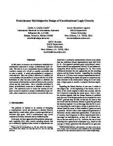
31000 30000 29000 28000 27000 26000 25000 24000 23000 22000 23000 24000 25000 26000 22000 27000 23000 24000 z1 28000 25000 29000 26000 27000 30000 28000 z2 29000 3000031000
Figure 3: A Comparison of the Noninferior Sets Obtained Using CMEA and BLP using SPEA-II, NSGA-II, and PESA. The performance metrics for SPEA-II, NSGA-II, and PESA are calculated based on 30 di�erent sets of solutions reported by Zitzler et al. (2001). Figure 3 compares the noninferior solutions generated by CMEA and the BLP solutions. The CMEA solutions appear to represent most of the noninferior surface de ned by the BLP solutions, which represent the best estimate of the noninferior front available for this problem. The extreme regions, associated with the three \tail-like" sections, are well represented by the CMEA solutions. Figures 4 to 6 compare the noninferior solutions generated by SPEA-II, NSGA-II, and PESA, respectively, with those generated by CMEA. The results from SPEA-II, NSGA-II, and PESA required approximately 576,000 function evaluations (Zitzler et al. 2001), and the CMEA solutions are based on approximately 594,000 function evaluations. While the solutions by SPEAII, NSGA-II, and PESA solutions well represent the \center" region of the noninferior surface, they entirely miss the three tail regions. The performance metrics listed in Table 1 were computed for the solutions generated by the MOEAs, and are compared in Figures 7 to 15. These graphs show for each metric the average and the range based on di�erent random trials. The Spread metrics in the three objective
SPEA-II CMEA
1
z3
0.8
Z1 spread
31000 30000 29000 28000 27000 26000 25000 24000 23000 22000
0.6
0.4
23000 24000 25000 26000 22000 27000 23000 24000 z1 28000 25000 29000 26000 27000 30000 28000 z2 29000 3000031000
0.2
0 CMEA
Figure 4: A Comparison of the Noninferior Sets Obtained Using CMEA and SPEA-II
SPEA-II
NSGA-II
PESA
Figure 7: Z1 spread comparison for CMEA, SPEA-II, NSGA-II, and PESA (a higher value indicates a better performance)
NSGA-II CMEA z3
31000 30000 29000 28000 27000 26000 25000 24000 23000 22000
22000
23000 24000 25000 26000 27000 23000 24000 z1 28000 25000 29000 26000 27000 30000 28000 z2 29000 3000031000
Figure 5: A Comparison of the Noninferior Sets Obtained Using CMEA and NSGA-II PESA CMEA z3
31000 30000 29000 28000 27000 26000 25000 24000 23000 22000 23000 24000 25000 26000 22000 27000 23000 24000 z1 28000 25000 29000 26000 27000 30000 28000 z2 29000 31000 30000
Figure 6: A Comparison of the Noninferior Sets Obtained Using CMEA and PESA
spaces are shown in Figures 7 to 9. These gures indicate that CMEA outperforms the other algorithms compared in this study. Figure 10 compares the coverage metric V 2. While all MOEAs perform similarly, PESA shows a slight edge over the others. When comparing metric V 1 in Figure 11, CMEA clearly outperforms the other MOEAs. This con rms the observations (from Figures 4 to 6) that SPEA-II, NSGA-II, and PESA solutions cover only the central region of the noninferior surface while the CMEA solutions are broadly distributed. Comparisons of C factors are shown in Figures 12 and 13. This further con rms the conclusions drawn above about coverage based on the V 1 and V 2 metrics. Comparisons of D-factor are shown in Figures 14 and 15. By collectively interpreting the values of DCMEA/another MOEA and Danother MOEA/CMEA for each MOEA compared, it can be concluded that CMEA solutions dominate those of the other MOEAs to a higher degree than vice versa. Alternatively, it implies that when CMEA solutions dominate solutions of another MOEA, they dominate them to a higher degree than when solutions of another MOEA dominate solutions of CMEA.
0.8
1
0.7
0.9
0.6
0.8
0.5
Metric V2
Z2 spread
1.1
0.7 0.6
0.3
0.5
0.2
0.4
0.1
0.3 CMEA
SPEA-II
NSGA-II
0
PESA
Figure 8: Z2 spread comparison for CMEA, SPEA-II, NSGA-II, and PESA (a higher value indicates a better performance)
CMEA
1
0.8
0.9
0.7
0.8
0.6
0.7
0.5
0.6
0.3
0.4
0.2
0.3
0.1
CMEA
SPEA-II
NSGA-II
PESA
Figure 9: Z3 spread comparison for CMEA, SPEA-II, NSGA-II, and PESA (a higher value indicates a better performance)
NSGA-II
PESA
0.4
0.5
0.2
SPEA-II
Figure 10: Coverage metric V 2 comparison for CMEA, SPEA-II, NSGA-II, and PESA (a lower value indicates a better performance)
Metric V1
Z3 spread
0.4
0 CMEA
SPEA-II
NSGA-II
PESA
Figure 11: Coverage metric V 1 comparison for CMEA, SPEA-II, NSGA-II, and PESA (a lower value indicates a better performance)
0.25
1 0.2 0.8
D factor
C factor
0.15 0.6
0.1 0.4 0.05 0.2 0 CMEA/SPEA-II
0 SPEA-II
NSGA-II
CMEA/NSGA-II
CMEA/PESA
PESA
Figure 12: Comparison of C factor: CMEA solutions over SPEA-II, NSGA-II, and PESA solutions
Figure 14: Comparison of D factor: CMEA solutions over SPEA-II, NSGA-II, and PESA solutions (a larger value indicates a higher degree of dominance of CMEA over another MOEA)
0.25
1 0.2 0.8
D factor
C factor
0.15 0.6
0.1 0.4 0.05 0.2 0 SPEA-II/CMEA
0 SPEA-II
NSGA-II
NSGA-II/CMEA
PESA/CMEA
PESA
Figure 13: Comparison of C factor: SPEA-II, NSGA-II, and PESA solutions over CMEA solutions
Figure 15: Comparison of D factor: SPEA-II, NSGA-II, and PESA solutions over CMEA solutions (a larger value indicates a higher degree of dominance of another MOEA over CMEA)
5
Conclusions
Comparing the noninferior solutions obtained using SPEA-II, NSGA-II, and PESA with those obtained using BLP (which is the best available estimate of the noninferior surface), CMEA performs relatively well in nding noninferior solutions that are close to the best available estimation, as well as in covering most of the noninferior surface for the thee-objective extended knapsack problem. When comparing the solutions obtained by the di�erent MOEAs tested in this study, CMEA performs better than all others with respect to the spread of solutions in the noninferior space. While CMEA solutions are able to cover a broader portion of the noninferior surface, the other MOEAs generate a high density of solutions in the central portion of the noninferior surface. In the context of accuracy or degree of dominance, the CMEA solutions dominate those generated by the other MOEAs relatively more frequently. While this study provides a systematic comparison of several MOEAs for only one three-objective optimization problem, further testing and evaluation studies are needed. Similar to the large array of test problems used in two-objective MO optimization, additional three-objective test problems re ecting di�erent problem complexities need to be de ned and be used in further comparative studies of these MOEAs. Also, the scale-up implications of higher number of objectives on the computational needs of the di�erent MOEAs need to be investigated. 6
Acknowledgments
The authors would like to thank Dr. Eckart Zitzler for sharing their results obtained using NSGA-II, SPEA-II, and PESA for the test problem reported in this paper. References
Corne, D. W., J. D. Knowles, and M. J. Oates (2000). The pareto-envelope based selec-
tion algorithm for multiobjective optimixation. In S. et al. (Ed.), Parallel Problem Solving from Nature - PPSN VI, Lecture Notes in Computer Science, pp. 869{878. Springer Verlag. Deb, K. (2001). Multi-objective Optimization Using Evolutionary Algorithms. England: John Wiley and Sons, Ltd. Deb, K., A. Pratap, and T. Meyarivan (2000). A fast elitist non-dominated sorting genetic algorithm for multiobjective optimization: NSGA-II. In Proceedings of the Parallel Problem Solving from Nature VI, pp. 849{858. Kumar, S. V. (2002). Vitri - A Generic Framework for Engineering Decision Support
on
Heterogeneous
Computer
Net-
. Ph. D. thesis, North Carolina State University. Ranjithan, S. R., S. K. Chetan, and H. K. Dakshina (2001). Constraint methodbased evolutionary algorithm (CMEA) for multiobjective optimization. In E. Z. et al. (Ed.), Evolutionary Multi-Criteria Optimization 2001, Lecture Notes in Computer Science 1993, pp. 299{313. SpringerVerlag. Zitzler, E., M. Laumanns, and L. Thiele (2001). Improving the strength pareto evolutionary algorithm. Technical Report 103, Computer Engineering and Communications Networks Lab (TIK), Swiss Federal Institute of Technology (ETH), Zurich, Gloriastrasse 35, CH-8092. Zitzler, E. and L. Thiele (1999). Multiobjective evolutionary algorithms: A comparative case study and the strength pareto approach. IEEE Transactions on Evolutionary Computation 2 (4), 257{271. works