Evaluation of Thresholding Techniques For Segmenting Scaffold ...

Evaluation of Thresholding Techniques For Segmenting Scaffold Images In Tissue Engineering Srinivasan Rajagopalan, Michael J. Yaszemski, M.D., Ph.D., Richard Robb Ph.D., Mayo Clinic/Foundation, Rochester, Minnesota, USA. ABSTRACT Tissue engineering attempts to address the ever widening gap between the demand and supply of organ and tissue transplants using natural and biomimetic scaffolds. The regeneration of specific tissues aided by synthetic materials is dependent on the structural and morphometric properties of the scaffold. These properties can be derived nondestructively using quantitative analysis of high resolution microCT scans of scaffolds. Thresholding of the scanned images into polymeric and porous phase is central to the outcome of the subsequent structural and morphometric analysis. Visual thresholding of scaffolds produced using stochastic processes is inaccurate. Depending on the algorithmic assumptions made, automatic thresholding might also be inaccurate. Hence there is a need to analyze the performance of different techniques and propose alternate ones, if needed. This paper provides a quantitative comparison of different thresholding techniques for segmenting scaffold images. The thresholding algorithms examined include those that exploit spatial information, locally adaptive characteristics, histogram entropy information, histogram shape information, and clustering of gray-level information. The performance of different techniques was evaluated using established criteria, including misclassification error, edge mismatch, relative foreground error, and region nonuniformity. Algorithms that exploit local image characteristics seem to perform much better than those using global information. Keywords: Tissue Engineering, scaffolds, microCT, thresholding.

1. INTRODUCTION Millions of surgical procedures requiring organ (tissue) substitutes to repair or replace malfunctioning organs (tissues) are performed worldwide every year. The ever widening gap between the demand and supply of transplant organs (tissues) has resulted in seeking natural and biomimetic solutions. Autografting, allografting and tissue engineering techniques are currently pursued to carry out transplantation. Autografting involves harvesting a tissue from one location in the patient and transplanting it to another part of the same patient. Though autologous grafts typically produce the best clinical results, primarily due to minimal rejection, they have several associated problems including procurement morbidity, additional surgical cost for the harvesting procedure, and infection and pain at the harvesting site. Allografts involve harvesting tissue or organs from a donor and then transplanting it to the patient. Minor immunogenic rejection, risk of disease transmission, and shortage of donors severely limits allografts. Tissue engineering involves regenerating damaged or malfunctioning organs from the recipient's own cells. The cells are placed in a tissue culture where they multiply. Once enough number of cells are produced they would be embedded

on a carrier material, scaffold, that is ultimately implanted at the desired site. Since many isolated cell populations can be expanded in vitro using cell culture techniques, only a small number of healthy cells is necessary to prepare such implants. On implantation and integration, blood vessels attach themselves to the new tissue, the scaffold dissolves, and the newly grown tissue eventually blends in with its surroundings. This technology has been effectively used to create various tissue analogs including skin, cartilage, bone, liver, nerve and vessels [1]. In spite of the projected benefits of engineered tissues, their percentage share in transplantation procedures is low. For example, of the 450,000 (20% of worldwide 2.2 million) bone grafts performed annually in the US, autogenous bone was used in 60% compared with 34% allografts and 6% engineered tissues [2]. Though there has been rapid progress in the field of Tissue Engineering since this 1996 statistics, the percentage share of tissue engineered grafts has not increased tremendously. This is partly due to the following hurdles reminiscent of an evolving technology. •

Material requirements: The scaffold material has to be non-mutagenic, non-antigenic, non-carcinogenic, nontoxic, non-teratogenic, highly bio-compatible and depending on the need - biodegradable or bioresorbable or bioabsorbable.

•

Manufacturing Practices: Depending on the importance of the final shape of the scaffold, they could be either injected or preformed. When the final shape is not important or is defined by local in vivo environment, the use of injectable and in situ forming scaffolds is important. Preformed scaffolds are useful when the final shape is important. The main functions of these scaffolds are to • • • •

Provide timely mechanical support and stability Define and maintain a 3D space for the formation of a new tissue Guide the development of a new tissue to achieve the appropriate functions Localize and deliver the cells to a specific site in the body upon implantation.

Preformed structural scaffolds are formed from structural elements such as pores, fibers or membranes. These elements are ordered according to stochastic, fractal or periodic principles and can also be manufactured reproducibly using rapid prototyping approaches like Solid Freeform Fabrication (SFF). Conventional scaffold fabrication techniques include fiber bonding, phase separation, solvent casting, particulate leaching, membrane lamination, melt molding, gas foaming, high pressure processing, hydrocarbon templating, freeze drying etc. [3]. These techniques typically produce stochastically ordered pores and have been used to engineer a variety of tissues. Manual intervention, inconsistent and inflexible processing procedures, use of toxic organic solvents, use of porogens, shape limitations and irreproducibility are the main limitations of these techniques. Figure 1 shows candidate MicroCT sections of scaffolds produced by particulate leaching technique. SFF techniques are computerized fabrication techniques that can rapidly produce complex three-dimensional objects using data generated by CAD systems, medical imaging modalities and digitizers [4]. Customized design, computer-controlled fabrication, and reproducibility are the main advantages of SFF techniques. However, current cookie-cutting approaches lead to bulk degradation of scaffold material. Hence the coordination of the scaffold biodegradation rate with the native tissues' biosynthetic rate is a major obstacle in these techniques. Moreover, unit cells (building blocks) of scaffolds are constructed typically using Boolean operations of geometric objects. Such unit cells, when tessellated to form the final scaffold might not yield functionality similar to a monolithic structure.

Figure 1: Candidate microCT sections of a scaffold produced using particulate leaching technique

•

Quantitation Techniques: While rapid advances are being made to overcome the abovementioned material and manufacturing hurdles, there are also concurrent efforts to understand the ramifications of the structure and spatial gradient of the scaffolds. The regeneration of specific tissues aided by synthetic materials has been shown to be dependent on diverse characteristics like pore size, porosity, pore shape, pore interconnectivity, material surface chemistry, effective scaffold permeability and scaffold stiffness [5] of the scaffolds. A large surface area enables cell attachment and growth, whereas a large pore volume is required to accommodate and subsequently deliver a cell mass sufficient for tissue repair. Highly porous biomaterials are also desirable for the easy diffusion of nutrients to and waste products from the implant and the vascularization that are major requirements for the regeneration of highly metabolic organs such as liver and pancreas. The surface area/volume ratio of porous materials depends on the density and average diameter of the pores. Theories of Padera and Colton [6] and Rosengren [7] establish the dependence of vascular penetration on implant pore size. Whang et al [8] and Klawitter et al [9] have experimentally arrived at optimum pore size of 5 microns for neovascularization, 5-15 microns for fiberblast ingrowth, 20 microns for ingrowth of hepatocytes, 100-350 microns for regeneration of bone, and about 500 microns for fibrovascular tissues. Another important consideration is the continuity of the pores within a synthetic matrix. Materials transport and cell migration will be inhibited if the pores are not connected even if the matrix porosity is high [10]. Cells more than

approximately 200 microns from a blood supply are either metabolically inactive or necrotic due to low oxygen tension [11]. Besides pore size and porosity, the shape and tortuosity can affect tissue ingrowth [12]. The scaffold should have the mechanical strength needed for creation of a macroporous scaffold that will retain its structure after implantation, particularly in the reconstruction of hard, load-bearing tissues, such as bones and cartilages. The biostability of many implants depend on factors such as strength, elasticity, absorption at the material interface and chemical degradation.

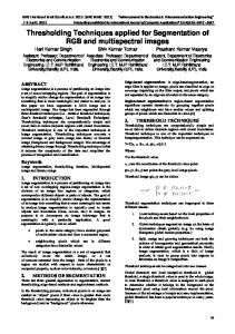
Quantitative analysis of these contributing factors is needed to validate the fabrication process and meet the mandated good manufacturing practices prescribed by regulatory bodies (FDA, CE). While there is a general intuitive consensus that these characteristic factors influence tissue regeneration, their specific magnitudes are loosely defined. The structural and functional characteristics of the scaffolds can be derived quantitatively from their three-dimensional microCT scans. However, the significance of the computed characteristics depends largely on the accuracy of the method used to identify the pore and polymeric phase. Since the scaffolds are usually produced using stochastic processes, visual thresholding is not guaranteed to produce accurate classification. Automatic thresholding algorithms give different results based on the assumptions made therein. Figure 2 shows the effect of varying the threshold values in the calculation of porosity (fraction of void space to total space) and the number of connected component which is a measure of interconnectivity. Porosity and interconnectivity index are the primary indices from which secondary indices could be derived subsequently [13]. The graphs clearly indicate the sensitivity of primary indices and consequently to the secondary indices to the polymer/pore threshold selected. Existing attempts [14,15] to quantify porous scaffolds do not address this issue adequately. In [14], the authors use the same threshold value on a set of differently fabricated scaffold images. Hence there is a strong motivation to investigate different thresholding techniques for segmenting polymeric and pore phases in scaffold images.

Figure 2: Effect of thresholding on scaffold porosity and interconnectivity. The graphs clearly indicates the sensitivity of the primary indices to the selected threshold

2. IMAGE THRESHOLDING TECHNIQUES: A BRIEF OVERVIEW In many applications of image processing, the gray levels of pixels belonging to the object are distinctly different from the gray levels of pixels belonging to the background. Thresholding then becomes a simple but effective tool to separate objects from the background [16]. Mathematically, a threshold operator can be viewed as a test for evaluating a function F of the form F(x,y), L(x,y), g(x,y)) where (x,y) indicates the spatial location of a pixel, L(x,y) denotes some local property of the pixel and g(x,y) is the gray level of the pixel at (x,y). If an image is partitioned into smaller subimages and a threshold is determined for each subimages by evaluating F, the threshold is referred to as local threshold. If the thresholding is based on the whole image, then it is referred to as global threshold. Global thresholds could be further classified into point-dependent and region-dependent. In Point-dependent techniques, the threshold is decided only on the basis of intensity distribution g(x,y). Region-dependent approaches make us of both the g(x,y) and the local property L(x,y). The main difficulty associated with thresholding occur when the associated noise process is non-stationary, correlated and non-gaussian. In addition, ambient illumination, variance of gray levels within the object and the background, inadequate contrast, and the lack of objective measures to assess the performance of a number of different thresholding algorithms also limit the reliability of an automatic thresholding algorithm. There are a number of survey papers on thresholding especially with respect to document binarization. Lee [17] suggested several criteria for evaluating thresholding performance and used them to compare five global methods. Trier [18] compared nineteen different methods to segment characters from documents with complex backgrounds. Sahoo [19] critiqued nine different algorithms and Glasbey [20]. Based on the image characteristics used to binarize (or even n-arize) images, the thresholding methods could be broadly grouped as follows: o o o o o o

Histogram shape-based methods which are based on the analysis of smoothed histogram of an image. Clustering-based methods in which the gray level samples are clustered into background and foreground. Entropy-based methods which compute the entropy of the foreground-background regions and the cross entropy between the original and binarized images. Fuzzy-logic based methods which measure the similarity between the original and thresholded image using fuzzy similarity measures Global methods which take into consideration the correlation between pixels on a global scale. Local methods which adapt the threshold value regionally depending on the local image characteristics.

3. THRESHOLDING METHODS FOR SCAFFOLD IMAGES Towards evaluating the ability of different algorithms to correctly segment scaffold images, we implemented a number of algorithms belonging to all the groups mentioned above. Specifically, we implemented 1.

Histogram shape-based method of Rosenfeld [21] that is based on analyzing the concavity points of the convex hull of the probability mass function of the image. The deepest concavity points of the convex hull are potential candidates for the threshold. The selection among the concavity points for the optimum threshold is based on

attributes like low busyness of the thresholded image which could be modeled as T = arg max{|max[p(I) – Hull(p(I)]} where p(I) is the probability mass function (pmf) of the image I and Hull() is the convex hull of the pmf of I. 2.

Iterative thresholding of Riddler [22]. This method models the gray level distribution in an image as a mixture of two Gaussian distributions representing, respectively, the background and foreground regions. At iteration i, a new threshold Ti is established using the average of the foreground and background class means. Iteration stops when the change |Ti – Ti+1| becomes sufficiently small.

3.

Clustering thresholding of Otsu [23] which minimizes (maximizes) the weighted sum of intra-class variances (interclass scatter) of the foreground and background pixels to establish an optimum threshold.

4.

Minimum error thresholding of Lloyd [24] which assumes that the image can be modeled by a mixture distribution of foreground (fg) and background (bg) pixels ie. p(g) = P(T) * pfg(g) + (1-p(T)).pbg(g) where P(T) is the cumulative probability from 0 to T. Assuming equal variance Gaussian density function, the thresholding that minimizes the total misclassification error is computed as

 m fg (T ) + mbg (T )  1 − P (T )  σ2  Topt = arg min  + log m fg (T ) − mbg (T ) 2   P (T )  where σ2 is the variance of the whole image and mfg(T) and mbg(T) are the mean of the foreground and background regions respectively obtained at threshold T.

5.

Minimum error thresholding of Kittler [25]. Though this method also assumes Gaussian distribution of the foreground and background class conditional probability density functions, it does not assume the variance to be equal. Consequentlty, the optimal threshold is estimated as:

Topt = arg min[ P(T ) log σ fg (T ) + (1 − P(T )) log σ bg (T ) − P(T ) log P(T ) − (1 − P(T )) log(1 − P(T ))] where σfg(T) and σbg(T) are the foreground and background variances respectively for a given threshold T.

6.

Entropy based thresholding of Kapur [26]. In this method the foreground and background classes are treated as two different sources. The image is considered to be optimally thresholded when the sum of the two class entropies reaches a maximum. Thus given foreground and background entropies defined as

 p (i )  p (i )  and H fg (T ) = − ∑ log  i = 0 P (T )  P (T )  T

H bg (T ) = −

G

p (i )

 p (i ) 

∑ P(T ) log  P(T ) 

i =T +1

Topt = arg max[Hfg(T) + Hbg(T)]





7.

Spatial thresholding based on two-dimensional image entropy [27]. This method considers the joint entropy of the image intensity value, g, at a pixel and the average intensity value, gav, of a small neighborhood centered at that pixel.

8.

Nonlinear dynamic window thresholding of White [28]. In this method the gray value of the pixel is compared with the average of the gray values in a small neighborhood. If the pixel is significantly darker than the average, it is assigned as foreground; otherwise it is classified as background.

9.

Local thresholding of Niblack [29]. This method adapts the local threshold according to the local mean and standard deviation over a window of size mxn. The threshold at pixel(i,j) is calculated as T(ij) = m(i,j) + Kσ(i,j) where m(i,j) and s(i,j) are the local sample mean and variance respectively. We used a window size of m=n=10 and a bias setting of k= -0.3 in our experiments.

10. Local thresholding of Bernsen [30]. The local threshold is set at the minimum and maximum of a local window taking into consideration that the contrast over the local window is beyond a certain threshold. 11. Local thresholding using surface fitting approach of Yanowitz [31]. This method is based on the combining the edge and gray-level information to construct a threshold surface. The image gradient magnitude is obtained and thinned to yield local gradient maxima. The threshold surface is constructed by interpolation with potential surface functions over successive over-relaxation method. The threshold is obtained as: Tn(i,j) = Tn-1(i,j) + Rn(i,j)/4 where R(i,j) is the discrete Laplacian of the surface. 12. Indicator kriging method of Oh [32]. This two-pass, hybrid method combines global and local estimates of the threshold. In the first pass, using global thresholding techniques, majority of the pixel population is assigned to either foreground or background based on their distinct deviation from the global threshold. In the second pass, the remaining pixels that are close to the global threshold are assigned to either of the classes using local covariance of the class indicators and the constrained linear regression.

4. RESULTS AND QUANTITATIVE ANALYSIS Figure 3 shows the results of segmenting candidate scaffold slices using the twelve methods described in the previous section. The number beneath each image indicates the method described in section 3 which produced the corresponding result. As expected, the local methods, with exception to the method of Bernsen (# 10), performed better than others. Bernsen method’s performance was limited by the inadequate contrast in the pore-polymer interface. However, among global methods, Otsu’s approach (#3) performed equally well. Riddler’s approach (#2), true to its assumption, isolated the background from the scaffold, thereby creating a ‘scaffold mask’. The minimum error thresholding of Lloyd (#4) is a multi-level thresholding algorithm and hence classified the salt from the polymeric phase. Visually, the indicator kriging method (#12) seemed to produce the best segmentation. For quantitatively evaluating these results, we computed the accuracy measures (False Negative, False Positive, and True Positive volume fractions) described in [33]. The estimation of these fractions depends on the availability of ground truth. Since it is impossible to get absolute ground truth for scaffolds created by stochastic processes, we manually “classified” each pixel into pore and polymer to create surrogate ground truth. Due to the large dimensions

(290x360x250) of the scaffold images, surrogate ground truth was created for a subset of the sections and accuracy measures were restricted to these sections. Table 1 shows the computed accuracy measures for each of the methods.

Figure 3: Qualitative comparison of scaffold pore/polymer segmentation with twelve different algorithms. Numbers below each figure indicates the result of the algorithm described in Section 3.

The accuracy measures reported in the table agree with our qualitative visual evaluation. To further quantitate the results, we computed the porosity for the scaffold based on each of these classifications and compared it to the measured porosity based on mercury porosimetry [34]. The computed porosity values are reported in the last column of Table 1. Mercury porosimetry experiment on this scaffold yielded a porosity of 68%. The computed values seem to be in line with the statistical measures.

Method #

TPVF

FPVF

FNVF

1 3 5 6 7 8 9 10 11 12

48.22 89.87 47.85 35.78 62.17 89.87 88.43 39.09 93.79 98.68

22.26 0.21 27.14 0.08 15.93 0.21 0.27 0.01 0.28 0.87

51.78 10.13 52.14 64.22 37.83 10.12 11.57 60.91 6.2 1.32

Jaccard similarity 39.44 86.69 37.63 35.76 62.07 89.69 85.23 39.05 93.54 98.27

Dice similiarity 56.57 92.9 54.69 52.68 76.60 94.56 92.03 56.17 96.66 99.13

Computed Porosity 32.84 61.3 32.48 24.29 43.4 61.1 60.2 27.3 64.5 66.9

Table 1: Accuracy measures and Computed Porosity for the different thresholding algorithms

5. CONCLUSIONS

In this paper we have reviewed a spectrum of thresholding algorithms to segment microCT images of polymeric scaffolds. Algorithms that exploit the local characteristics of the image clearly outperform the global methods. This highlights the pitfalls in the current practice of visually estimating the pore-polymer thresholds leading to inaccurate characterization of scaffolds. This could be one of the reasons why seemingly good scaffolds perform badly on implantation and integration at the native site. One of the drawbacks in our evaluation strategy, that is also innate to a majority of evaluation strategies, is the need to create surrogate ground truth. Alternate strategies that are free of ground truth needs to be explored.

6. REFERENCES [1] Lanza P.P., Langer R., Vacanti J., Principles of Tissue Engineering. Academic Press 2000. [2] Boyce T., Edwards J., Scarborough N., “Allograft bone: the influence of processing on safety and performance”, Orthop. Clin. N.Am, 1999:30:571-581. [3] Yang S., Leong K.F., Du Z., Chua C.K., “Design of scaffolds for use in Tissue Engineering: Part I Traditional Factors”, Tissue Engineering 2001:7(6):679-689. [4] Hutmacher D.W., “Scaffold Design and Fabrication Technologies for Engineering Tissues: State of Art and Future Prospectives”, J.Biomater. Sci. Polymer Edn., 2001:12(1):107-124. [5] Cima LG, Vacanti JP, Vacanti C, et al. “Tissue engineering by cell transplantation using degradable polymer substrates”, J. Biomech Eng. 113, 143, 1991. [6] Padera RF, and Colton CK, “Time Course of Membrane Microarchitecture-Driven Neovascularization”, Biomaterials, 17:277-284, 1996. [7] Rosengren A, Danielsen N and Bjursten LM, “Reactive Capsule Formation around Soft-Tissue Implants is related to Cell Necrosis”, J. Bio Mat Res, 46(4):458-464, 1999. [8] Whang K, Healy E, Elenz DR et al., “Engineering bone regeneration with bioabsorbable scaffolds with novel microarchitecture”, Tissue Eng., 5, 35, 1999. [9] Klatwiller JJ and Hulbert SF, “Application of porous ceramics for the attachment of load-bearing internal orthopedic applications ”, J. Biomed. Mater. Res. Symp. 2, 161, 1971.

[10] Moone DJ, Baldwin DF, Suh NP et al., “Novel approach to fabricate porous sponges of poly(D,L-lacto-co-glycolic acid) without the use of organic solvents”. Biomaterials 17, 1417, 1996. [11] Colton CK, “Implantable biohybrid artificial organs”, Cell transplant. 4, 415, 1995. [12] Mooney D, Hansen L, Vacanti J et al., “Switching from differentiation to growth in hepatocytes: control by extracellular matrix”, J.Cell Physiol. 51, 497, 1992. [13] Lin A.S.P., Barrows T.H., Cartmell S.H., Guldberg R.E., “Microarchitectural and Mechanical Characterization of Oriented Porous Polymer Scaffolds”, Biomaterials, 24:481-489, 2003. [14] HilderbrandT, Laib A, Muller R, et al., “Direct three-dimensional morphometric analysis of human cancellous bone: microstructural data from spine, femur, iliac crest and calcaneous”, J. Bone Miner Res, 14(7):1167-74, 1999. [15] Filmon R., et al. “Non-connected versus interconnected macroporosity in poly(2-hydroxyethyl methacrylate) polymers. An X-ray microtomographic and histomorphometric stud”, J.Biomater. Sci. Polymer Edn. 13(10):1105-1117, 2002. [16] Weszka JS, and Rosenfeld A, “Threshold evaluation techniques”, IEEE Trans. Sys. Man Cybernet. SMC-8:622629, 1978. [17] Le SU, Chung SY, Park A, “A comparative performance study of several global thresholding techniques for Segmentation”, Graphical Models and Image Processing, 52:171-190, 1990. [18] Trier OD, Jain AK, “Goal-directed evaluation of binarization methods”, IEEE Trans. PAMI, 17:1191-1201, 1995. [19] Sahoo PK, Soltani S, Wong AKC, Chen Y, “A survey of thresholding techniques”, Computer Graphics and Image Processing, 41:233-260, 1988. [20] Glasbey CA, “An analysis of histogram-based thresholding algorithms”, Graphical Models and Image Processing, 55:532-537, 1993. [21] Rosenfeld A, Torre P, “Histogram Concavity analysis as an aid in threshold selection”, IEEE Trans System, Man and Cybernetics, SMC-13:231-235, 1983. [22] Ridler TW, Calvard S, “Picture thresholding using an interative selection method”, IEEE Trans System, Man and Cybernetics, SMC-8:630-632, 1978. [23] Otsu N, “A threshold selection method from gray level histograms”, IEEE Trans System, Man and Cybernetics, SMC-9:62-66, 1979. [24] Lloyd DE, “Automatic target classification using moment invariance of image shapes”, Technical Report, RAE IDN AW 126, Farnborough-UK, Deember 1985. [25] Kittler J, Illingworth J, “Minimum Error Thresholding”, Pattern Recognition, 19:41-47, 1986. [26] Kapur JN, Sahoo AKC, Wong A, “A new method for gray-level picture thresholding using the entropy of the histogram”, Graphical models and Image Processing, 29:273-285. 1985. [27] Abutaleb AS “Automatic Thresholding of Gray-level Pictures using Two-dimensional entropy” Computer Vision Graphics and Image Processing, 47:22-32, 1989. [28] White JM, Rohrer GD, “Image Thresholding for Optical Character Recognition and other applications requiring character image extraction”, IBM J. Res. Development, 27(4):400-411, 1983. [29] Niblack W, An introduction to Image Processing, Prentice Hall pp. 115-116, 1986. [30] Bernsen J, “Dynamic Thresholding of Grey level images”, In Proc. Intnl. Conf. On Pattern Recognition, ICPR’86. pp:1251-1255, 1986. [31] Yanowitz SD, Bruckstein AM, “A new method for image segmentation”, Computer Graphics and Image Processing, 46:82-95, 1989. [32] Oh W, Lindquist B, “Image thresholding by indicator kriging”, IEEE Trans. Pattern Analysis and Machine Intelligence, PAMI-21:590-602, 1999. [33] Udupa J.K. et al, "A methodology for Evaluating Image Segmentation Algorithms" In Proc. SPIE, 4684:266-277, 2002. [34] J. van Brakel (ed.), Powder Technol., 29:1-209, 1981.