Is Agricultural Production Becoming More or Less Sensitive to Extreme Heat? Evidence from U.S. Corn and Soybean Yields
Michael J. Roberts and Wolfram Schlenker
Abstract Extreme heat is the single best predictor of corn and soybean yields in the United States. While average yields have risen continuously since World War II, we find no evidence that relative tolerance to extreme heat has improved between 1950 and 2005. Climate change forecasts project a sharp increase in extreme heat by the end of the century, with the potential to significantly reduce yields under current technologies.
We would like to thank James Bushnell and Catherine Wolfram for helpful comments. This material is based upon work supported in part by the Department of Energy under Grant No. DE-FG02-08ER64640 and the National Science Foundation under Grant No. 0962559.
North Carolina State University. Email:
[email protected] Columbia University and NBER. Email:
[email protected]
1. The Role of Agriculture in the US Economy The share of employment in the agricultural sector in the United States has been continuously declining. About half of the occupations in the 1870 Census were classified as agriculture, and a significant share of the workforce in the manufacturing and service sector were related to agriculture.1 In the 2000 Census, only 1.9 percent of the workforce was employed in agriculture, forestry, fishing, hunting, or mining. Employment in the agricultural sector decreased by 1.8% per year in the postwar period 1947-1985, while agriculture exhibited one of the highest post-war productivity growth rates of 1.6% per year, only surpassed by communications (Jorgenson and Gollop, 1992). Growth in agricultural productivity is shown in Figure 1, which displays yields for corn, soybeans, and wheat for the years 1866-2009.2 It shows yearly outcomes as well as trend lines. Before World War II, yields were stable over time and production increases were driven by expansion of the growing area into the Western United States. Following World War II, growth switched from the extensive to the intensive margin: output per acre increased significantly due to new seed varieties and increased use of fertilizer while the growing area stabilized and even declined slightly.3
In addition to yield growth, productivity was enhanced with steadily
improving farm equipment, which allowed each farmer to manage increasingly larger growing areas. On a global scale, supply growth outpaced demand growth causing commodity prices to decline in real terms over the 20th century. Today, at least in relatively developed nations, agriculture’s share of GDP is small. Estimates vary depending on how much of food processing and distribution is included in the calculation. In the United States it is comparable to its employment share, i.e., about 2 percent. Given the small share of GDP that is attributable to agriculture in the United States, some people have argued that climate change does not pose a significant threat. There are, however, three reasons why changing climate conditions might still be economically meaningful. First, 1
Table 26: 6 out of 12.5 million occupations were classified as agriculture.
2
www.nass.usda.gov. The time series for soybeans does not start until 1924.
3
The exception is soybeans, a relatively new crop that is grown in rotation with corn, which showed area increase throughout the 20th century.
while agriculture constitutes a small share of GDP, it accounts for a large share of consumer surplus. Demand for agricultural goods is highly inelastic (Roberts and Schlenker, 2010). A shortage of food has the potential to cause large price increases, as was evident in the fourfold price increase in staple commodity prices between 2005 and 2008.
Second, agricultural
production depends directly on weather fluctuations and is more susceptible to changing climatic conditions than other sectors of the economy. In contrast, most manufacturing today occurs within buildings, thereby insulating the process from weather fluctuations unless extreme events keep inputs or the workforce from reaching the plant. Third, agriculture in the United States is important because it constitutes a large share of global production. Corn, rice, soybeans, and wheat comprise about 75 percent of the caloric consumption of humans (Cassman 1999). The United States share of caloric production among these four commodities has been relatively constant at around 23 percent for the last forty years. This share is about twice as large as Saudi Arabia’s share of world oil production (13 percent of world total, US Energy Information Administration).4 Given its sheer size, any impact on US agricultural production can have large repercussion on world food markets.5
And for less developed nations, food expenditures
comprise a much larger share of national income.
2. The Effect of a Changing Climate on Agricultural Output Economic studies have used both cross-sectional and panel data to empirically study potential effects of climate change on agriculture. Cross-sectional studies typically associate climate with land values (Mendelsohn et al. 1994, Schlenker et al. 2006) while panel studies link agricultural output to year-to-year weather fluctuations (Deschenes and Greenstone 2007, Schlenker and Roberts 2009).
Each of these approaches has strengths and weaknesses.
Cross-sectional
differences in current climate can capture how farmers adapt to permanent difference in climate, 4 5
http://www.eia.doe.gov/emeu/cabs/Saudi_Arabia/Oil.html The United States is generally predicted to experience larger temperature increases than the global average. Despite non-uniform temperature increases, Battisti and Naylor (2009) observe that equatorial regions have a greater likelihood of experiencing temperatures that are outside the historic range since historic weather variation has also been lower. This makes statistical identification of weather and climate effects for off-equatorial zones more plausible because larger historic variations can be used to estimate a model and predicted climate change impacts do not require large out-of-sample extrapolations.
yet they can be susceptible to omitted variables and specification biases. On the other hand, year-to-year weather fluctuations are plausibly random and exogenous to farm decision making, but cannot account for long-run adaptation, and thus may over- or underestimate effects of climate change depending on whether the set of possible adaptation choices are larger in the long-term or short-term. Both approaches are incapable of capturing equilibrium effects; that is, they effectively assume all prices remain constant. We first summarize earlier findings in Section 2.1. We present the average effect of various weather variables in Section 2.2, and examine the evolution of the key variables over time in Section 2.3.
2.1 The Importance of Extreme Heat on Agricultural Output – Earlier Results In previous work we found similar relationships between corn or soybean yields and temperatures using three distinct sources of identification: (i) a 56-year panel of yields from 1950-2005; (ii) a cross-section linking average yields to average weather outcomes; (iii) and a time series linking annual yields to annual weather outcomes (Schlenker and Roberts, 2009). Temperature effects were modeled using a flexible functional form: yields are increasing in temperature up to 29C (84F) for corn and 30C (86F) for soybeans, but further temperature increases are harmful to yields. The ideal growing condition would be a constant temperature of 84F for corn and 86F for soybeans.
Deviations from this optimal temperature result in
approximately linear yield reductions. This linearity is captured by the concept of degree days, which are the number of degrees above a baseline, summed over all days for the growing season. For example, a temperature of 34C with a baseline of 30C would result in 4 degree days, while all temperatures below 30C would results in zero degree days. In the following we use the data and optimal bounds from Schlenker and Roberts (2009), i.e., all counties east of 100 degree longitude, an approximate boundary between the irrigated west and the dryland east.6 The exception is Florida, which is excluded as most counties are highly irrigated. As a first step we use a panel data set to estimate.7
6
The 100 degree meridian roughly cuts Texas in half in the east-west dimension.
7
In all regressions but column (5) of Table 1 the errors are clustered by state.
2.2 Average Relationship between Weather and Yields The baseline model is yit = αi + β1 hit + β2 mit + β3 pit + β4 pit2 + ts + ts2 + εit
(1)
where yit are log corn or soybean yields in county i in year t, αi is a county fixed effect, mit captures moderate temperatures (degree days 10-29C for corn and degree days 10-30C for soybeans), hit extreme heat (degree above 29C for corn and degree days above 30C for soybeans), pit precipitation (in cm), and ts and ts2 are state-specific quadratic time trends. Results from estimation equation (1) are reported in Table 1. The first column of the table uses only the measure of extreme heat and omits all other weather variables. The second column adds additional weather variables for moderate heat and precipitation. The third column uses area-weights (amount of cropland in each county) in the regression, while the fourth column uses all counties from the United States as opposed to just the Eastern subset. While previous research has argued that the response function is different in irrigated areas, adding them in a pooled model has limited effects as the irrigated crop area is small and therefore receives little weight. Column (5) uses only the time series in the identification where both the dependent variable yt and exogenous weather variables are averaged over all counties in the sample and cropland area-weights are used: yt = α + β1 ht + β2 mt + β3 pt + β4 pt2 + t + t2 + εt
(2)
Column (6), considers only the cross-section and uses the model yi = αi + β1 hi + β2 mi + β3 pi + β4 pi2 + εi
(3)
where yi is the average difference of the yield in a county from the overall log yield in that year, i.e., yi = 1/T t(yit-yt), and the weather variables are averages over the 56 years. All coefficients have the expected sign: Deviations from optimal precipitation levels (both too little and too much) are harmful. An increase in moderate heat (shifting from cold temperatures to moderate temperatures) is beneficial while an increase in extreme heat is detrimental. Climate change is predicted to move the temperature distribution upwards. Shifting the lower (cooler) part of temperature distribution towards the optimum temperature of 29C or 30C is beneficial, but the effects are dwarfed by the damaging effects of more frequent temperatures above the optimum. The dominating factor that drives predicted yield impacts is
the measure of extreme heat as (i) the magnitude of the coefficient in the first row of Panel A and B of Table 1 are large, and (ii) the measure of extreme heat is predicted to increase significantly in higher latitudes as described in the previous section. Each 24-hour exposure to each degree above 29C for corn and 30C for soybeans lowers annual yields by 0.4 to 0.7 percent. In other words, if a plant is exposed 24 hours to 40C, yields decrease by about 5 percent. The most striking feature of these results is that they are similar whether we use the time series in column (5) or the cross-section in column (6). While the former measures the effect of year-to-year weather shocks to which farmers can only partially adapt as they are realized after the plants have been sown, the latter compares how places with different average growing conditions have adapted to them. It seems quite unlikely that unobserved factors might confound the cross-sectional relationship in a manner that causes it to spuriously match the same nonlinear relationship observed in the time series.
2.3 The Evolution of Heat and Drought Tolerance over Time Given the high sensitivity of yields to extreme temperatures, one might wonder whether there has been progress in developing plants that are more resistant to extreme heat over time. Average yields improved greatly over our 56-year time frame. But what happened to heat tolerance? In Roberts and Schlenker (2009) we examined the evolution of the weather-yield relationship over the entire 20th century in the state of Indiana, including such extreme events as the Dust Bowl in the 1930s. Here, we focus on the more recent past (1950-2005), but instead use a richer geographic coverage. To answer this question we generalize specifications reported in column (2) of Table 1 by allowing the coefficients to vary over time. The model is: yit = αi + fh(t) hit + fm(t) mit + fp(t) pit + fp2(t) pit2 + ts + ts2 + εit
(4)
where f(t) includes a constant plus restricted cubic splines of time.8 The results for fh(t) are shown in the top row of Figure 2 and 3, while the results for fp2(t) are shown in the bottom row. Recall that the average coefficients were given in column (2) of Table 1. These figures plot how two of these coefficients evolve over time.9 Each figure shows the results for all counties east of the 100 degree meridian (except Florida) in the left column, while the second and third column 8
We use 5 knots as the baseline but obtain comparable figures if we use 7 knots instead.
9
Results for the remaining two coefficients on moderate heat and precipitation are available on request.
limit the sample to the cooler northern and warmer southern subset of states, respectively.10 Each graph also lists the p-value for an F-test that the splines are jointly different from zero, implying that the coefficient of interest evolves over time. The only significant change in heat tolerance can be detected for northern subsample for corn and southern subsample for soybeans. Both suggest that heat tolerance decreased over time. On the other hand, the coefficient on the squared precipitation term, which measures the reduction in yield as precipitation deviates from the optimal level, is significant in most cases and generally shows an upward trend, which indicates crop yields have become less sensitive to fluctuations in precipitation.
2.4 Policy Implications Why do corn and soybean show large improvements in average yields and better resistance to precipitation fluctuations, yet show no improvement or even a worsening in heat tolerance? One reason might be that greater heat tolerance comes partially at the expense of reduced yield potential. Wahid et al. (2007) emphasize that “acquiring thermotolerance is an active process by which amounts of plant resources are diverted to structural and functional maintenance to escape damages caused by heat stress.” Presumably, those resources would otherwise go into seed formation and greater yields in the event of less extreme weather. At the same time, heat tolerance and drought tolerance are inherently intermingled because water requirements increase with temperature. A plant wilts because it did not receive enough water for a given level of heat, or it received too much heat for a given amount of water. While plants require more water when temperatures go up, historic weather data in the United States has shown the opposite association: there is a negative correlation between extreme heat and precipitation in the 56-year time series in Table 1 as evaporation following rainfall results in cooling. This helps to explain the highly damaging effect of extreme heat in the historic time series: water requirements increase with extreme heat, yet water availability generally decreases as it only gets very hot once the soils are dry. But some effects of extreme heat act separately
10
Northern states are Illinois, Indiana, Iowa, Michigan, Minnesota, New Jersey, New York, North Dakota, Ohio, Pennsylvania, South Dakota, and Wisconsin. Southern states are Alabama, Arkansas, Georgia, Louisiana, Mississippi, North Carolina, Oklahoma, South Carolina, Tennessee, and Texas.
from water availability. For example, regardless of water availability, corn does not flower if temperatures are too high. Breeding new crop varieties is a long-term process. Alston et al. (1992) review the history of crop research, which traditionally has been publicly funded, especially in developed countries. The economic rationale for a public role in basic research is that there are positive spillovers from the spread of ideas, so private companies do not necessarily have the right incentives to breed the most socially beneficial crops, as they cannot reap all the benefits. In the United States, the Morrill Act and the Hatch Act created Land Grant universities in the second half of the 19th century with a mission to teach and study agriculture and created a cooperative extension service to interact with farmers. On an international level, the Consultative Group on International Agricultural Research (CGIAR) has several research centers around the world designed to improve yields of plants that are native to a region. Norman Borlaug, a previous director at CGIAR’s International Maize and Wheat Improvement Center in Mexico received the Nobel Peace Prize for his work in improving yields and avoiding starvation. The Bill and Melinda Gates Foundation set out to become a CGIAR center and assist in reforming the agency as recent articles have highlighted that the budget for various CGIAR centers, e.g., the International Rice Research Institute, have been cut significantly as world production outpaced demand and led to a downward drift in prices until 2005.11 Alston et al. (1992) note that recently private companies have taken over a larger share of research and development. One reason for growing interest from private companies is that bioengineering can allow seed companies generate more productive seed that do not reproduce, thereby enhancing excludability.12 Herbicide resistance, a key trait in the first generation of commercial genetically modified crops, also complements other products owned by seed companies. Some biotechnology companies have reported success in developing new strains with increased drought tolerance, yet critics have argued that such success has been reported
11
“World’s Poor Pay Price as Crop Research Is Cut,” New York Times, May 18, 2008.
12
Seed companies might still have problems capturing all the rent from innovation if a drastic innovation significantly lowers production cost (Gallini and Wright, 1990).
before but did not materialize in the field.13 There is little documented evidence on increased heat tolerance that is not counterbalanced by reduced yield potential. Recent food price spikes have shown the most detrimental consequences of reduced supply fall on people living in poorest countries who can no longer afford food consumption when prices start to rise. The problem is not necessarily a shortage of caloric production, but large income disparities. The taste for meat in developed countries, which requires many more calories in production, might price poor people out of the market and lead to famine. On the other hand, many remain optimistic about the potential of genetically modified crops, which might usher a new era of innovation that breaks historical the tradeoff between heat tolerance and yield potential. To date most commercially successful genetically modified crops resist pests or herbicides. But more ambitious efforts exist to develop plants that manufacture their own nitrogen fertilizer and possess more nutrients. These innovations, among others, would be especially beneficial to poor countries. While public funding of basic research has diminished, private donations from charities like the Gates Foundation or by profit-driven companies like Monsanto might replace these funds. But given public good attributes of research, there remain important questions about the extent to which private incentives to fund basic research align with potential social welfare.
3 Conclusions This paper considers how changing climatic conditions may affect agricultural output and how heat tolerance has evolved over time. Changing climate conditions, specifically the increased frequency of extreme heat, has the potential to significantly decrease yields of staple crops in the United States that form an important basis of caloric consumption. Since the United States is by far the world’s largest producer and exporter of commodity calories, this has the potential to impact world prices of staple food commodities. One big question is whether advances in biotechnology might increase heat tolerance enough to make crops more resistant to extreme heat. On the upside, crops have become less susceptible to precipitation fluctuations. On the downside, the recent trend has been towards varieties with higher average yields with unchanged or even more sensitive to extreme heat. This suggests that the kind of technological change 13
“Drought Resistance Is the Goal, but Methods Differ.” New York Times, October 22, 2008.
needed to cope with a warming climate would be historically unprecedented. The changes needed differ markedly from the kind of technological changes that has brought about the green revolution—a three- to four-fold increase in yields that as occurred since World War II. Comparative advantages will obviously change with the climate. Thus, the most natural and least-cost form of adaptation would seem to involve simply changing the locations where agricultural activities take place. However, the best soil is found in currently moderate temperate zones, thereby limiting the potential to shift to higher latitudes. How all the shifts will add up globally remains highly uncertain.
References Alston, Julian M., Philip G. Pardey and Johannes Roseboom. 1992. “Financing Agricultural Research: International Investment Patterns and Policy Perspectives.” World Development, 26(6): 1057-1071. Battisti, David. S. and Rosamond L. Naylor. 2009. “Historical Warnings of Future Food Insecurity with Unprecedented Seasonal Heat.” Science, 323(5911): 240-244. Cassman, Kenneth G. 1999. “Ecological intensification of cereal production systems: Yield potential, soil quality, and precision agriculture.” Proceedings of the National Academy of Sciences, 96(11): 5952-5959. Deschenes, Olivier and Michael Greenstone. 2007. “The Economic Impacts of Climate Change: Evidence from Agricultural Output and Random Fluctuations in Weather.” American Economic Review, 97(1): 354-385. Gallini, Nancy T and Brian D. Wright. 1990. “Technology Transfer under Asymmetric Information.” Rand Journal of Economics, 21(1): 147-160. Houghton, R. A., J. L. Hackler, and K. T. Lawrence. 1999. “The U.S. Carbon Budget: Contributions from Land-Use Change.” Science, 285(5427): 574-578. Jorgenson, Dale W. and Frank M. Gollop. 1992. “Productivity Growth in U.S. Agriculture: A Postwar Perspective.” American Journal of Agricultural Economics, 74(3): 745-750. Mendelsohn, Robert, William D. Nordhaus, and Daigee Shaw. 1994. “The Impact of Global Warming on Agriculture: A Ricardian Analysis.” American Economic Review, 84 (4): 753-771. Roberts, Michael J. and Wolfram Schlenker. 2009. ““The Evolution of Heat Tolerance of Corn: Implications for Climate Change,” NBER Conference Volume: Climate Change - Past and Present. Roberts, Michael J. and Wolfram Schlenker. 2010. “Identifying Supply and Demand Elasticities of Agricultural Commodities: Implications for the US Ethanol Mandate.” NBER Working Paper 15921. Schlenker, Wolfram, Anthony C. Fisher, and W. Michael Hanemann. 2006. “The Impact of Global Warming on U.S. Agriculture: An Econometric Analysis of Optimal Growing Conditions.” Review of Economics and Statistics, 88(1): 113-125. Schlenker, Wolfram and Michael J. Roberts. 2009. “Nonlinear Temperature Effects Indicate Severe Damages to U.S. Crop Yields under Climate Change.” Proceedings of the National Academy of Sciences, 106(37): 15594–15598. Whalid, A., S. Gelani, M. Ashraf, and M. R. Foolad. 2007. “Heat tolerance in plants: An overview.” Environmental and Experimental Botany, 61(3): 199-223.
Figure 1: Corn, Soybean, and Wheat Yields in the United States (1866-2009)
Notes: Graphs shows yields over time (1866-2009 for corn and wheat and 1924-2009 for soybeans). Yearly observations are shown as scatter plot and a nonparametric trend line is added (Epanechnikov kernel with a bandwidth of 10 years).
Figure 2: The Effect of Extreme Heat and Precipitation on Corn Yields (1950-2005)
Notes: Graphs display the effect of extreme heat (top row) and precipitation (bottom row) on corn yields over time. The left column uses all counties east of the 100 degree meridian (except for Florida), while the second and third column use only the northern and southern subsets, respectively.
Figure 2: The Effect of Extreme Heat and Precipitation on Soybean Yields (1950-2005)
Notes: Graphs display the effect of extreme heat (top row) and precipitation (bottom row) on soybean yields over time. The left column uses all counties east of the 100 degree meridian (except for Florida), while the second and third column use only the northern and southern subsets, respectively.
Extreme Heat Moderate Heat Precipitation Precipitation Squared Observations
Table 1: The Effect of Weather on Corn and Soybean Yields (1) (2) (3) (4) Panel A: Corn -0.594*** -0.637*** -0.746*** -0.700*** (0.054) (0.070) (0.048) (0.056) *** *** 0.043 0.040*** 0.031 (0.007) (0.007) (0.007) *** *** 1.681 1.48*** 1.031 (0.217) (0.338) (0.345) *** *** -0.008 -0.015 -0.013*** (0.002) (0.003) (0.003) 105981 105981 105981 120995
(5)
(6)
-0.639*** (0.114) 0.034* (0.018) 3.963** (1.658) -0.039*** (0.015) 56
-0.410*** (0.135) 0.002 (0.020) 3.544 (2.555) -0.035 (0.021) 2275
Panel B: Soybeans Extreme Heat -0.541 -0.581 -0.586*** -0.583*** -0.395*** -0.380*** (0.031) (0.029) (0.040) (0.039) (0.089) (0.129) *** *** *** 0.040 0.039 0.022 0.005 Moderate Heat 0.040 (0.005) (0.007) (0.007) (0.013) (0.012) Precipitation 1.222*** 1.275*** 1.244*** 1.224 0.864 (0.166) (0.206) (0.200) (1.517) (1.69) Precipitation Squared -0.009*** -0.010*** -0.010*** -0.011*** -0.009 (0.001) (0.002) (0.002) (0.013) (0.013) Observations 82385 82385 82385 85225 56 2078 Subset East East East US East East Area-weighted No No Yes Yes No No Notes: Table regresses log yields on weather variables for the months March-August. All coefficients are multiplied by 100, so they roughly report the effect of each variable in percent. Extreme heat is measured by degree days above 29C for corn and degree days above 30C for soybeans. Moderate heat is measured by degree days between 10C and 29C for corn, and 10 and 30C for soybeans. Precipitation is the season total and measured in cm. Columns (1)-(4) use a panel of yields, while column (5) uses the time series (average yield and weather in a year) and column (6) uses the cross-section (average yield and weather in a county). Errors are clustered in STATA at the state level. ***
***