Evolution of Neural Architecture Fitting Environmental Dynamics Genci Capi Fukuoka Institute of Technology, Japan Kenji Doya ATR, Computational Neuroscience Laboratories Temporal and sequential information is essential to any agent continually interacting with its environment. In this paper, we test whether it is possible to evolve a recurrent neural network controller to match the dynamic requirement of the task. As a benchmark, we consider a sequential navigation task where the agent has to alternately visit two rewarding sites to obtain food and water after first visiting the nest. To achieve a better fitness, the agent must select relevant sensory inputs and update its working memory to realize a non-Markovian sequential behavior in which the preceding state alone does not determine the next action. We compare the performance of a feed-forward and recurrent neural control architectures in different environment settings and analyze the neural mechanisms and environment features exploited by the agents to achieve their goal. Simulation and experimental results using the Cyber Rodent robot show that a modular architecture with a locally excitatory recurrent layer outperformed the general recurrent controller. Keywords non-Markovian sequential task · recurrent neural network · evolutionary algorithm · evolved behavior
1
Introduction
Execution of a complex sequence of actions is a challenge even for humans and primates. It is surprising that even the tiny brain of an insect is capable of producing highly complex sequential behaviors, such as in foraging, homing, and mating. The performance of sequential tasks is associated with activation of diverse areas in the brain and requires the storage and update of internal states. Instead of arbitrary connection topology, we often find modular organization in the brain. For example, the most prominent feature of the architecture of the
cerebral cortex is its columnar organization; neurons stacked on top of each other through the depth of the cortex tend to be connected and have similar response properties despite residing in different layers (Fujita, Tanaka, Ito, & Cheng, 1992). Columnar organization is also found in the prefrontal cortex, which plays a major role in working memory (Kritzer & GoldmanRakic, 1995). Cerebellum also has modular organization called micro-zones. The main motivation of this paper is to understand the origin of locally excitatory, laterally inhibitory modular organization of the brain. Recurrent neural networks, which operate not only on an external space but also on an internal state space,
Correspondence to: G. Capi, Department of System Management, Fukuoka Institute of Technology, 3-30-1 Wajiro-Higashi, Higashi-ku, Fukuoka, 811-0195, Japan. E-mail:
[email protected] Tel.: +81-92-606-5892, Fax: +81-92-606-0756.
Copyright © 2005 International Society for Adaptive Behavior (2005), Vol 13(1): 53–66. [1059–7123(200503) 13:1; 53–66; 050134]
53
54
Adaptive Behavior 13(1)
are able to represent (and learn) temporal/sequential extended dependences over unspecified (and potentially infinite) intervals. Fully-connected recurrent networks have universal computational capacity, but actually training them to perform a complex dynamic function is quite difficult. The specific question we consider in this paper is whether modularly organized recurrent networks have advantage over fully-connected recurrent networks in the evolution of complex dynamic functions. To test such a hypothesis, we used a self-excitatory, laterally inhibitory recurrent neural network as the simplest model of modular network. In connectionist studies, supervised learning algorithms have been applied to recurrent neural networks (Doya, 2002). Despite encouraging early results in training simple neural oscillators and state machines (Doya & Yoshizawa, 1989; Pearlmutter, 1989; Williams & Zipser, 1989), it has turned out to be very difficult to train a network to process complex sequences with long-range interactions (Bengio, Simard, & Frasconi, 1994; Doya, 1995), although by fine tuning the architecture and parameters, it is not impossible (Hochreiter, 1997; Rodriguez, 2001). Reinforcement learning algorithms have also been applied to recurrent neural networks for control of locomotion (Sato, Nakamura, & Ishii, 2002) and sequential behaviors (Nakahara, Doya, & Hikosaka, 2001; Faihe & Muller, 1997; Jones & Mataric, 1998). Evolution of recurrent networks has also been explored for locomotion (Mathayomchan & Beer, 2002) and sequential behaviors (Meeden, 1996; Urzelai & Floreano, 2001). For example, Urzelai and Floreano (2001) evolved neural controllers for a Khepera robot to travel back and forth between lighted and dark target areas, using proximity, light and visual sensors. Tuci, Quinn, and Harvey (2002) demonstrated that it is possible to evolve an integrated dynamic neural network that successfully controls an agent engaged in a simple learning task where the robot learns the relationship between the position of a light source and the location of its goal. The networks have fixed synaptic weights and leaky integrator neurons. Yamauchi and Beer (1996) showed that continuous time recurrent neural networks capable of sequential behavior and learning can be evolved to display reinforcement learning-like abilities. The task studied was generation and learning of short bit sequences based on reinforcement from the environment. Blynel (2003) further extended this work to an artificial agent task where a simulated Khepera robot has to navigate first in a simple and then a double T-maze.
Unlike previous approaches, in the experiments reported here, we consider a much more complex nonMarkovian sequential task in which the memory of a preceding event alone does not determine the next action to be taken. Therefore, in addition to ordinary working memory of the most recent event, the agent must store and update a higher-order working memory. In addition, in order to compare the performance of arbitrary and modular topologies, and evolution considering the weight connections, topology and connectivity of neural controllers. The task is for a Cyber Rodent (CR) robot (Capi, Uchibe, & Doya, 2002; Elwing, Uchibe, & Doya, 2003) to navigate between three places, marked by different colors, in a given order: food–nest–water–nest–food– nest–water–nest–…. After visiting the food, water or nest, the CR faces the problem of what to do next. This issue, often termed action selection, continues to be a major concern of biology, ethology, and neuroscience. Seth (1998) advocates the position that action selection does not depend upon internal arbitration and also on any kind of internalization of behavior. Based on arguments from ethology, Blumberg (1994) shows that greater control over the temporal aspects of behavior and the need for a flexible means of modeling the influence of internal and external factors are important aspects of any action-selection mechanism. On the other hand, research in neuroscience shows that basal ganglia appears to be related with action selection (Redgrave, Prescott, & Gurney, 1999). We compare the performance of different control architectures in order to understand the neural mechanisms and environment features exploited by the agents to achieve their goal. The performance is tested in stationary and non-stationary environments with different relative positions between the landmarks. We considered the performance of a feed-forward neural network (FFNN) controller and two recurrent neural networks: A globally-recurrent neural network (GRNN), also known as Elman’s network (Elman, 1990), and a locally-recurrent neural network (LRNN), which has memory units with self-excitation and lateral inhibition. We used a real-valued GA to set the connection weights as well as the number of hidden and memory units. The results show that the FFNN performed fairly well when the locations of food, water, and nest were fixed throughout the course of evolution. Therefore, there was no need to rely on explicit internal memory. However, in the second environment, when the posi-
Capi & Doya Neural Architecture and Environmental Dynamics
55
Figure 1 Neural architectures. (a) the FFNN with one hidden layer. (b) The GRNN architecture is similar to Elman’s recurrent network. (c) The LRNN contains a memory layer where neurons with self-excitation and lateral inhabitation receive inputs from the input layer.
tions of food and water were changed during agent life, agents with FFNN performed badly. GRNN also failed to capture the higher-order structure of the sequence; LRNN gave the best performance by successfully switching between two levels of memory and by utilizing local recurrent connections. The output of memory units showed a strong correspondence with the agent’s next goal. In order to assess robustness, the neural controllers evolved in simulation were then tested in the real hardware of the CR robot. Despite their differences, especially with regard to timing, the robot performed the sequential navigation task well.
The inputs of neural controllers are the angle to the nearest landmark (food, water or nest), three units (R, G, B) for color-coding of the nearest landmark, and three tactile sensor units (food, water or nest), each of which is activated only when the agent reaches the landmark according to the sequential order. The egocentric angle to the nearest landmark varies from 0 to 1 where 0 corresponds to 45° to the right and 1 to 45° to the left. The hidden, memory and output units use sigmoid activation functions 1 y i = ---------------1 + e –xi
2
(1)
Evolving Dynamic Networks where incoming activation for node i is
2.1 Neural Architectures The FFNN, GRNN and LRNN control architectures are shown in Figures 1a–c, respectively. The FFNN has one hidden layer. The GRNN architecture is similar to Elman’s recurrent network, where the hidden unit activation values are copied back and used as extra inputs in the next time step. The LRNN contains a memory layer where neurons with self-excitation and lateral inhibition receive inputs from the input layer. Unlike other works (Paul, 2003), the neural networks do not have bilateral symmetry.
xi =
∑ wji yj
(2)
j
and j ranges over nodes with weights into node i. The output of memory units of LRNN is 0 or 1, based on activation and threshold value as follows: 1 if y mem ( i ) ≥ thresh ( i ) . y mem ( i ) = 0 if y mem ( i ) < thresh ( i )
(3)
56
Adaptive Behavior 13(1)
Figure 2 Genetic encoding of neural architectures. (a) The genome of FFNN encodes the weight connections and the number of hidden neurons. (b) The genome of GRNN encodes the weight connections, number of hidden neurons and their initial values. (c) The genome of LRNN encodes the weight connections, thresholds and initial values of memory neurons, interconnection between memory neurons and the number of hidden and memory units.
The output units directly control the right and left wheel angular velocities where 0 corresponds to no motion and 1 corresponds to full-speed forward rotation. The left and right wheel angular velocities, ωright and ωleft, are calculated as follows: ωright = ωmax * yright ω left = ωmax * yleft
(4)
where ωmax is the maximum angular velocity and yright and yleft are the neuron outputs. The maximum forward velocity is considered to be 0.5 m/s. 2.2 Genetic Encoding The genome of every individual of the population is designed to encode the structure of each neural controller. In our GA, in addition to the weight connections between the units, we also optimized the number of hidden and memory units varying between 1 and 5. Figure 2a–c presents the genomes of FFNN, GRNN and LRNN, respectively. The maximum genome length of the FFNN controller is 46. The first 35 genes encode synaptic weights of input-to-hidden connections, while the next 10 genes encode those of hidden-to-output
connections, and the last gene encodes the number of hidden units (Figure 2a). The respective genome lengths of GRNN and LRNN are 76 and 147. The GRNN genome includes weight connections (35 for input-to-hidden, 10 hidden-to-output and 25 memory units-to-hidden), initial values of memory units (5) and the number of hidden units (1) (Figure 2b). The LRNN genome encodes synaptic weights (35 for input-tohidden, 10 hidden-to-output and 35 input-to-memory, 25 interconnected memory units, 25 memory-to-output), thresholds (5) and initial values of memory units (5). In addition, one gene for each memory unit determines whether the neuron has self- and lateral connections (Figure 2c). The last two genes encode the number of hidden and memory units. The range of input, self- and lateral connection weights ranged from –10 to 10, 0 to 10 and –10 to 0, respectively. Rather than using variable-length genotypes to allow varying numbers of hidden and memory neurons, we use fixed-length genotypes with the maximum number of hidden and memory nodes. When the number of hidden or memory units is smaller than the maximum, some parts of the genome are ignored in constructing a phenotype network. Based on the number of hidden and memory units, the mutation operators are modified, such that mutated genes are always functional.
Capi & Doya Neural Architecture and Environmental Dynamics
57
Table 1 Real-number GA functions and parameters.
Function name Arithmetic crossover Heuristic crossover
Figure 3 Environment used in the simulation is a square of 5 m × 5 m.
2 [2 3]
Simple crossover
2
Uniform mutation
4
Non-uniform mutation
[4 GNmax 3]
Multi-non-uniform mutation
[6 GNmax 3]
Boundary mutation Normalized geometric selection
3
Parameters
4 0.08
Non-Markovian Foraging Task
3.1 Food–Nest–Water–Nest Task The task for the CR robot is to alternately visit food and water locations after first visiting the nest. The agent must learn low-level reactive responses. In addition, the agent must have working memory to reach the specific landmark according to the sequential order. When the agent visits the nest, a higher order memory level is needed to remember if the previous visited landmark was food or water. Figure 3 shows the simulated agent in the environment, which is a square of 5 m × 5 m. The food, water and nest are placed randomly in the environment, where the distance between them varies from 1.8 m to 2.3 m. In the simulated environment, 5% noise was added to the calculated angle of the nearest landmark. We considered the performance of neural controllers in different environmental settings. In the first environment, food, water and nest are fixed during the agent’s life and throughout generations. In the second setting, the food and water positions change after one third of the evaluation time and then change back after two thirds. In simulated environments, food, water and nest positions are considered squares of 0.05 × 0.05 m and their respective colors are red, blue and green, enabling the agent to distinguish them. 3.2 Evaluation and Evolution The CR robot is initially placed in a random position and orientation. Each individual of the population con-
trols the agent during a lifetime of 100 seconds (50 ms × 2000 time steps). The agent receives a positive reward of 1 if the visited position matches the sequential order, and is penalized by –1 otherwise. The individuals are selected for crossover and mutation operations based on their performance. A real-value GA was employed in conjunction with the selection, mutation and crossover operators. The genes, which encode the number of nodes, are also considered as real numbers. In the fitness function, they are converted to the upper bound integers. Many experiments comparing real-value and binary GA show that real-value GA generates superior results in terms of the solution quality and CPU time (Michalewich, 1994). The GA selection, mutation and crossover functions and their respective parameters are presented in Table 1 and a detailed explanation is given in the Appendix. Initially, 500 individuals were randomly created. The evolution terminated after 100 generations.
4
Simulation Results
This section presents the performance of neural controllers evolved in different environment settings. 4.1 Fixed Environment Figure 4 shows the performance of the agent controlled by FFNN. Under this environment setting, where the food nest and water are aligned almost linearly, the FFNN with three hidden neurons achieves fairy good
58
Adaptive Behavior 13(1)
Figure 4 Agent performance controlled by FFNN in fixed environment. When the food nest and water are aligned almost linearly, the FFNN achieves fairly good performance.
performance. Due to the lack of memory, the agent reaches any landmark that enters the field of its visual sensor. After moving to the food and then to the nest positions, the agent reaches the water place that happens to be within its field of vision. When the visual sensor detects no landmarks, the agent rotates clockwise, due to strong connection weights to the left wheel. After reaching the water position, the agent rotates clockwise and finds the food first. The agent then continues to rotate clockwise, and as soon as the nest becomes visible, it heads for this landmark. If the angle between the food and nest seen from the water location is larger than the agent’s view angle, the FFNN-controlled agent heads to the food and cannot complete the task according to the sequential order. Therefore, the performance of the neural controller depends on the relative positions of the landmarks. The GRNN and LRNN also solve the sequential task in fixed environments. Figure 5 shows the behavior of the agent controlled by GRNN. The agent does not find irrelevant landmarks after reaching the food position nor after reaching the nest coming from the food location. In addition, the agent reaches the nest
Figure 5 Agent performance controlled by GRNN in fixed environment. The agent always visits the landmarks according to the sequential order.
Figure 6 Average of fitness value shows that fitness of FFNN controller improved quickly during the first few generations. The average fitness of GRNN is higher than that of the FFNN controller. The LRNN fitness improves slower compared to other architectures, but achieved the best final performance.
coming from the food location in such a way that the food location would be visible only for a very short time, and the agent starts moving toward the water location. The agent ignores the food after reaching the water location. In a fixed environment, the easiest evolved strategy is to avoid seeing landmarks that do not match the sequential order by rotating in the direction such that the next visible landmark matches with the sequential order. When this is not possible, the agent has to ignore the next visible landmark. 4.2 Changing Environment In the changing environment, the evolved FFNN and GRNN neural controllers contained four units in the hidden layer, while the LRNN had three units in the hidden layer and four units in the memory layer. Three of the four units in the memory layer had lateral and self-connections, and one unit was not interconnected. The population average of fitness value of the three neural controllers is shown in Figure 6. The fitness during the first generations is low because there are agents which have no attraction to any landmark or only rotate passing through the same landmark many times. Based on the fitness value, these agents are removed from the population during the course of evolution. The fitness of the FFNN controller improved quickly during the first few generations and converged after 20 generations. The fast convergence of the FFNN was due to the short length of the genome and its evolved behavior. The average fitness of the GRNN is higher than that of the FFNN controller. The LRNN fitness improves more
Capi & Doya Neural Architecture and Environmental Dynamics
59
Figure 7 Performance of evolved neural controllers. The agent controlled by FFNN (a) reaches every landmark that becomes visible. At the beginning, the agent reaches the food position according to the sequential order. Then the agent visits the water place instead of nest, goes to the nest, then to the food instead of water. The GRNN agent (b) reaches according to the sequential order the food, nest, water, nest in the environment 1. When the environment changes, the agent ignores the water place and searches for the new food position. But after capturing the food position, the agent reaches the water place, which is not according to the sequential order. Then the agent reaches the nest position. In the environment 3, the agent continues to reach the landmarks according to the sequential order: Water, nest, food, nest, water, nest. The agent controlled by LRNN (c) always follows the sequential order. In the environment 1, the agent reaches the food, nest, water, and nest. When the environment changes (environment 2) the agent ignores the food position and after searching it reaches the new food position. The agent reaches the food, nest, water, and nest. In environment 3, the agent continues to reach the targets according to the sequential order: Food, nest, water, nest.
slowly than that of other architectures, but it achieved the best final performance. The GA is already converging after 80 generations. The trajectories of evolved FFNN, GRNN and LRNN controllers are shown in Figures 7a–c, respectively. Three different environments with different food and water positions are shown. The agent controlled by FFNN controller, due to its lack of memory, has the
worst performance (Figure 7a). The agent rotates in the environment and approaches whichever landmark appears in its visual sensor. The GRNN controller performs better. In the first and third environments, the agent successfully ignores the water and nest locations when it should reach the food. However, in the second environment, the agent reached the water before moving to the nest. Furthermore, after reaching the nest
60
Adaptive Behavior 13(1)
Figure 8 Neuron activation of LRNN. The activation of memory neurons shows that the first memory neuron is active when the agent has to visit the nest place. The third and fourth units specify whether to go to food and water, respectively. The second neuron is higher in the hierarchical level and deals with the higher order structure of the sequence.
from the food position it is again attracted by the food position (Figure 7b). Figure 7c shows the trajectory of the agent controlled by LRNN. The agent follows the sequential order in three different environments. When the food and water positions change, the agent that was heading toward the food ignores the water location in front and starts to search for and approach the new food position. Figure 8 illustrates the unit activation values of the LRNN. This figure shows how the agent utilized the angle and color of the nearest landmark and output of memory units in order to reach or avoid them. The activation of memory neurons shows that the first memory neuron is active when the agent has to visit the nest
place. The second neuron is higher in the hierarchical level and deals with the higher order structure of the sequence. The third and forth units specify whether to go to food and water, respectively. Thus, the agent acquired higher order working memory to deal with the nonMarkovian sequential order. The Hinton diagram of LRNN weight connections is shown in Figure 9. The memory units have strong connection weights with tactile units and self- and lateral connection weights. Therefore, the agent’s intention and switching between them is mainly achieved by tactile neurons and activation of memory units in the previous time step. The initial state of memory units is 0 0 1 0 and their respective threshold values are
Capi & Doya Neural Architecture and Environmental Dynamics
61
Figure 9 Hinton diagram for the memory-part of LRNN connection weights. The inputs are the angle, color (R, G, B), three tactile neurons (TF, Tw, TN) and activation of memory neurons in the previous time step. Activation of tactile units and memory units in the previous time step realize the switching between different agent’s intentions.
Figure 10 Agent performance controlled by LRNN when there is no reward for visiting the nest place. The agent always reaches the landmarks according to the sequential order. In the first and third environments, the agent avoids reaching the water place after moving close to it.
0.1723, 0.6572, 0.6621, and 0.7259. When the agent reaches the food place, the tactile unit TF is activated. Memory neuron M1 has a large positive weight with TF neuron and negative weight with M3. Because the positive connection is stronger than the negative one, and its threshold value is small, M1 becomes active. M3 loses activity because of negative connection between TF and M3 and small self-excitation. The strong positive connection of TF with M2 also activates the M2 neuron. Similar to the case discussed above, the activation of memory units changed, as shown in Figure 8. We also ran a new simulation in which we reduced the number of tactile units to 2. Each tactile unit was activated when the agent actually got food or water. We did not give reward for going back to nest; whether the right sequence was followed or not was informed only when the agent went to the food or water sites. This set-up replicated an experiment with real rats (Miyazaki, Miyazaki, Mogi, Matsumoto, & Tetsuya, 2002). In this environment set-up, the performance of agent controlled by FFNN and GRNN did not change.
The best LRNN controller had three neurons in the hidden layer and five neurons in the memory layer, where three of them have lateral and self-connections. The LRNN could complete the task (Figure 10) by utilizing the higher order memory coded in the memory layer. In the first and third environments, the agent shows some attraction to the water place, when before moving to the food position. Therefore, compared with the previous environment setting, the number of times the agent got food and water is slightly decreased. The agent utilized the visibility of nest position to switch its attention to food or water when visiting the nest position. Therefore, unlike the LRNN with three tactile units, the sensor encoding the landmark color has also strong connection weights with memory neurons.
5
Hardware Experiments
We implemented the evolved neural controllers, on the real hardware of the CR robot, which is a two-
62
Adaptive Behavior 13(1)
Figure 11 Two views of the Cyber Rodent robot used in the experiments.
wheel-driven mobile robot as shown in Figure 11. The CR is 250 mm long and weighs 1.7 kg. The CR is equipped with • • • • • • • • •
omni-directional C-MOS camera, IR range sensor, seven IR proximity sensors, 3-axis acceleration sensor, 2-axis gyro sensor, red, green and blue LED for visual signaling, audio speaker and two microphones for acoustic communication, infrared port to communicate with a nearby agent, wireless LAN card and USB port to communicate with the host computer.
Five proximity sensors are positioned on the front of the robot, one behind and one under the robot pointing downwards. The proximity sensor under the robot is used when the robot moves wheelie. The CR contains a Hitachi SH-4 CPU with 32 MB memory. The FPGA graphic processor is used for video capture and image processing at 30 Hz. The video capture of LRNN controller and the trajectory plot of CR motion are shown in Figures 12 and 13, respectively. The visual and proximity sensors in front of the CR robot are utilized to activate the input units when reaching the food, water or nest location according to the sequential order. Despite some differences due to the task and CR hardware specifications, the neural controller performed well. The noise in the calculated angle of the nearest landmark is reduced by a careful calibration of the camera (Capi et al., 2002). Because there were three different colors in the envi-
ronment, the FPGA needed time to analyze the captured image. Therefore, the sampling time needed to obtain the sensor data and calculate the wheel velocity was 90 ms. The proximity sensors readings are updated every 5 ms. Despite these differences, the CR robot completed the sequential task. The agent ignored irrelevant sensory inputs and reached the reward locations according to the sequential order, even when we changed the food and water locations.
6
Discussion
This article has explored the advantages of evolved modular neural architectures compared to arbitrary selected topologies for sequential tasks. We considered a non-Markovian sequential task, in which the agent had to obtain food and water after first visiting the nest. The task was interesting because the agent must: (1) Have working memory; (2) select relevant sensory inputs; (3) deal with the non-Markovian sequential order. Our analysis focused on the details of the internal workings of neural architectures and their relation with the behavior and environment dynamics. In particular, we demonstrated that LRNN outperformed the general recurrent neural controller by successfully switching between two levels of memory. By utilizing local recurrent connections, the LRNN performed better even in a more difficult and realistic environment set-up in which we reduced the number of tactile units. This brings us to suggest that modularly organized recurrent networks work better than fully connected recurrent networks for complex dynamic functions. This result is important not only to the field of evolutionary computation but also
Capi & Doya Neural Architecture and Environmental Dynamics
63
Figure 12 Video capture of CR robot controlled by LRNN. The agent continually reached the targets according to the sequential order even when the environment changed.
Figure 13
Trajectory plot of CR robot motion.
to the field of neuroscience as it provides a new perspective on the origin of modular topologies found in the brain, such as cortical columns and cerebellar microzones. The results show that there is a direct relationship between the agent intention and the output of memory units. The self-excitation and lateral inhibition of memory units has a great effect on the long-term working memory and appropriate time switching between different agent intentions. Based on the intention (output
of memory units) and landmark characteristics (color), the agent was able to decide to reach or avoid a visible landmark. The results of these experiments demonstrate that the evolutionary approach can scale up to the development of recurrent neural controllers, which are difficult to train using connectionist methods. In addition, the evolved recurrent controllers are able to perform robustly in varying and dynamic environmental conditions. The analyses considered different environment settings. In fixed environments, the agents controlled by general recurrent neural architectures completed the sequential task according to the sequential order. Although the agent must have an internal state to solve the task successfully, surprisingly, in some specific fixed environments even the agents controlled by FFNN gave good performance. The robustness of evolved neural controllers was also tested on the real hardware of CR robot, using the visual and proximity sensors. Although the time to process the visual information was longer, the evolved controllers performed well. This was mainly related to small noise in the input sensors. Some small differences between simulation and hardware trajectories were caused by the noise in the angle to the nearest landmark determined by the visual sensor.
64
Adaptive Behavior 13(1)
In our method, we evolved the weight connections and the neural controller topology. However, a disadvantage of our method is that chromosome length was considered fixed even when the number of hidden or memory units was small. Although we modified the genetic operators, it has to be tested whether a GA with variable length could give a better result in terms of CPU time. In addition, we would like to consider behavior adaptation in changing environments: For example, the case when the landmarks switch their colors during the agent life. Although there are some approaches in evolutionary computation or reinforcement learning, we are more interested in combining learning and evolution.
Appendix. Genetic Operators Used in Real-Number GA Selection Function Selection of individuals is done based on normalized geometric ranking, which defines selection probability pi for each individual as p i = q′ ( 1 – q ) r – 1
if i = j otherwise
(6)
where the ai and bi are the lower and upper bound of searching interval. The uniform mutation is repeated 4 times. Boundary mutation randomly selects one variable, j, and sets it equal to either its lower or upper bound, where r is uniform random number between (0, 1): ai ′ yi = bi xi
if i = j,
r < 0.5
if i = j,
r ≥ 0.5.
otherwise
y i′
x i + ( b i – x i )f ( G ) = xi –( xi + ai ) f ( G ) xi
if r 1 < 0.5 if i = j, r i ≥ 0.5,
(8)
otherwise
where b GN f ( G ) = r 2 1 – --------------- , GN max
with r1, r2 uniform random numbers between (0, 1), GN the current generation, GNmax the maximum number of generations, and b a shape parameter equal to 3. The multi non-uniform mutation operator applies the non-uniform operator to all of the variables in the parent X . Real-value simple crossover is identical to the binary version. Arithmetic crossover produces two complementary linear combinations of the parents, where r is uniform random number between (0, 1) as follows:
(5)
where q is the probability of selecting the best individual, r is the rank of the individual where 1 is the best, P is the population size, and q′ = q ⁄ ( 1 – ( 1 – q ) P ). Uniform mutation randomly selects one variable, j, and sets it equal to an uniform random number U(ai, bi) as follows: U ( a i, b i ) x i′ = xi
The boundary mutation is repeated 4 times. Non-uniform mutation randomly selects one variable, j, and sets it equal to a non-uniform random number:
(7)
X′ = rX + ( 1 – r )Y
(9)
Y′ = ( 1 – r )X + r Y .
(10)
Heuristic crossover produces a linear extrapolation of the two individuals. This operator utilizes the fitness information. A new individual, X′, is created using the following equation: X′ = r ( X – Y ),
(11)
Y′ = X,
(12)
where r is a uniform random number between (0, 1) and X is better than Y in term of fitness. If X′ is infeasible, i.e., feasibility equals 0 as given by 1 feasibility = 0
if x i′ ≥ a i, x i′ ≤ b i, ∀i otherwise
(13)
then generate a new random number r and create a new solution using (A7), otherwise stop. To ensure
Capi & Doya Neural Architecture and Environmental Dynamics
halting after t failures let the children equal the parents and stop. We considered t = 3. Simple crossover generates a random number r from a uniform distribution from 1 to m and creates two new individuals ( x′ and y′ ) according to the following equations: xi xi = yi yi yi = xi
if i < r otherwise if i < r otherwise
(14)
(15)
In Table 1, the parameter for arithmetic crossover, simple crossover, uniform mutation, boundary mutation and the first parameter of heuristic crossover, non-uniform mutation and multi-non-uniform mutation is the number of times to call the operator in every generation.
Acknowledgment The authors would like to thank the Japan Science and Technology Agency for supporting this project.
References Bengio, Y., Simard, P., & Frasconi, P. (1994). Learning long-term dependencies with gradient descent is difficult. IEEE Transactions on Neural Networks, 5(2), 157– 166. Blynel, J. (2003). Evolving reinforcement learning-like abilities for robots. In A. Tyrrell, P. C. Haddow, & J. Torresen (Eds.), Proceedings of 5th International Conference on Evolvable Systems: From Biology to Hardware (pp. 320– 331). Springer-Verlag GmbH. Blumberg, B. (1994). Action-selection in hamsterdam: Lessons from ethology. In D. Cliff, P. Husbands, J.-A. Meyer, & W. S (Eds.), From animals to animats 3: The Third International Conference on Simulation of Adaptive Behavior (pp. 108–117). Cambridge, MA: MIT Press. Capi, G., Uchibe, E., & Doya, K. (2002). Selection of neural architecture and the environment complexity. In K. Murase & T. Asakura (Eds.), International series on advanced intelligence: Vol. 6, Dynamic systems approach for embodiment and sociality (pp. 311–317). Doya, K. (1995). Recurrent networks: supervised learning. In M. A. Arbib (Ed), The Handbook of Brain Theory and Neural Networks (pp. 796–799). Cambridge, MA: MIT Press.
65
Doya, K. (2002). Recurrent networks: learning algorithms. In M. A. Arbib (Ed), The Handbook of Brain Theory and Neural Networks Cambridge, MA: MIT Press. Doya, K. & Yoshizawa, S. (1989). Adaptive neural oscillator using continuous-time backpropagation learning. Neural Networks, 2, 375–386. Elman, J. (1990). Finding structure in time. Cognitive Science, 14, 179–211. Elwing, S., Uchibe, E., & Doya, K. (2003). An evolutionary approach to automatic construction of the structure in hierarchical reinforcement learning. Proceedings of the Genetic and Evolutionary Computation Conference, (507–509). Springer-Verlag Berlin Heidelberg. Faihe, Y., & Muller, J. (1997). Analysis and design of robot's behavior: towards a methodology. In Proceedings of Sixth European Workshop on Learning Robot, Brighton, UK (pp. 46–61). London: Springer-Verlag. Fujita, I., Tanaka, K., Ito, M., & Cheng, K. (1992). Columns for visual features of objects in monkey inferotemporal cortex. Nature, 360, 343–346. Hochreiter, S., (1997). Recurrent neural net learning and vanishing gradient. In Proceedings of Fuzzy-Neuro Workshop, Soest, Germany. Jones, J., & Mataric, M. (1998). Sequential learning in minimalist neural network. In Proceedings of International Conference on Robotics and Automation (pp. 395–396). Kritzer M. F., & Goldman-Rakic P. S. (1995). Intrinsic circuit organization of the major layers and sublayers of the dorsolateral prefrontal cortex in the rhesus monkey. Comparative Neurology, 359(1), 131–143. Mathayomchan, B., & Beer, R. D. (2002). Center-crossing recurrent neural networks for the evolution of rhythmic behavior. Neural Computation, 14, 2043–2051. Meeden, L. A. (1996). An incremental approach to developing intelligent neural controllers for robots. IEEE Transaction on Systems, Man, and Cybernetics, 26, 474–485. Michalewich, Z. (1994). Genetic algorithms + data structures = evaluation programs. Berlin: Springer. Miyazaki, K., Miyazaki, K., Mogi, E., Matsumoto, G., & Tetsuya, K. (2002). Role of the nucleus accumbens neurons in goal-directed behavior. In Proceedings of the International Symposium on Limbic and Association Cortical Systems—Basic, Clinical and Computational Aspects, Toyama, Japan. Nakahara, H., Doya, K., & Hikosaka, O. (2001). Parallel cortico-basal ganglia mechanisms for acquisition and execution of visuomotor sequences—A computational approach. Journal of Cognitive Neuroscience, 13, 626–647. Nakamura, K., Sakai, K., & Hikosaka O. (1998). Neuronal activity in medial frontal cortex during learning of sequential procedures. Journal of Neurophysiology, 80(5), 2671–2687. Paul, C. (2003). Bilateral decoupling in the neural control of biped locomotion. In Proceedings of the Second Interna-
66
Adaptive Behavior 13(1)
tional Symposium on Adaptive Motion of Animals and Machines, Kyoto, Japan. Pearlmutter, B. A. (1989). Learning state space trajectories in recurrent neural networks. Neural Computation, 1, 263–269. Redgrave, P., Prescott, T. J., & Gurney, K. (1999). The basal ganglia: A vertebrate solution to the selection problem? Neuroscience, 89, 1009–1023. Rodriguez, P. (2001). Simple recurrent networks learn contextfree and context-sensitive languages by counting. Neural Computation, 13, 2093–2118. Sato, M., Nakamura, Y., & Ishii, S. (2002). Reinforcement learning for biped locomotion. In Proceedings of International Conference on Artificial Neural Networks (pp. 777– 782). Seth, A. K. (1998) Evolving action selection and selective attention without actions, attentions, or selection. In R.
Pfeifer, B. Blumberg, J. Meyer, & S. Wilson (Eds.), From animals to animats 5: Proceedings of the Fifth International Conference on the Simulation of Adaptive Behavior (pp. 139–147). Cambridge, MA: MIT Press. Tuci, E., Quinn, M., & Harvey, I. (2002). An evolutionary ecological approach to the study of learning behavior using a robot-based model. Adaptive Behavior, 10, 201–221. Urzelai, J., & Floreano, D. (2001). Evolution of adaptive synapses: robots with fast adaptive behavior in new environments. Evolutionary Computation, 9, 495–524. Williams R. J., & Zipser, D. (1989). A learning algorithm for continually running fully recurrent neural networks. Neural Computation, 1, 270–280. Yamauchi, B., & Beer, R. (1996). Sequential behavior and learning in evolved dynamical neural networks. Adaptive Behavior, 2(3), 219–246.
About the Authors Genci Capi took the B.E. and Ph.D. degrees from the Polytechnic University of Tirana and Yamagata University in 1993 and 2002, respectively. From April 2002 to March 2004, he was a Researcher at the Computational Neurobiology Department, ATR Computational Neuroscience Laboratories. Since April 2004 he has been an Assistant Professor in the Department of System Management, Fukuoka Institute of Technology. His research interests include intelligent systems, humanoid robots, learning and evolution. He is member of IEEE and Robotics Society of Japan (RSJ).
Kenji Doya took B.S. in 1984, M.S. in 1986, and Ph.D. in 1991 at the University of Tokyo. He became a Research Associate at the University of Tokyo in 1986, at the University of California San Diego in 1991, and the Salk Institute in 1993. He joined ATR in 1994 and is currently the Head of the Computational Neurobiology Department, ATR Computational Neuroscience Laboratories. In 2004, he was appointed as a Principal Investigator of Initial Research Project, Okinawa Institute of Science and Technology. He is interested in understanding the functions of basal ganglia and neuromodulators based on the theory of reinforcement learning. Address: 12-22 Suzaki, Gushikawa, Okinawa 904-2234, Japan. E-mail:
[email protected]