In many libre (free, open source) software projects, most of the development is performed by a relatively small num- ..... Symposium, Chicago, IL, USA, 2004.
Evolution of the core team of developers in libre software projects Gregorio Robles, Jesus M. Gonzalez-Barahona, Israel Herraiz GSyC/LibreSoft, Universidad Rey Juan Carlos (Madrid, Spain) {grex,jgb,herraiz}@gsyc.urjc.es
Abstract In many libre (free, open source) software projects, most of the development is performed by a relatively small number of persons, the “core team”. The stability and permanence of this group of most active developers is of great importance for the evolution and sustainability of the project. In this position paper we propose a quantitative methodology to study the evolution of core teams by analyzing information from source code management repositories. The most active developers in different periods are identified, and their activity is calculated over time, looking for core team evolution patterns.
1. Introduction Employee turnover is known to be high in the traditional software industry since many years ago [1]. However, in libre software1 projects the study of developer turnover has not been an active research topic. Most of the attention in this area has been focused on the organizational structure of the projects [2], with little attention to the dynamics of the developers. A noteworthy contribution in this sense, although it does not address the evolution of developer communities, is the onion model [3], which shows how developers and users are positioned in communities. In this model, it is possible to differentiate among core developers (those who have a high involvement in the project), codevelopers (with specific but frequent contributions), active users (contributing only occasionally) and passive users [4, 5]. This position paper shows how to better understand the evolution of the most active group of developers contributing to a libre software project. A specific methodology has been designed to quantitatively characterize a project in the spectrum between these two scenarios, and to visualize more in detail the evolution of the core team. The first steps of this methodology, applied to a few projects, are explained 1 In this paper we will use the term “libre software” to refer both to “free software” and “open source software”.
in [6]. An extension and refinement of the methodology is presented here.
2. Methodology The methodology used in this study is based on retrieving data about the activity of developers from source code management repositories, which are mined using CVSAnalY [7]. This tool retrieves information about every commit to the repository, and inserts it into a database where it can be conveniently analyzed. To characterize the evolution of the core team, first the life of the project is split in periods of equal duration. Then for every period i, the most active developers are identified as CoreT eami . This is done by calculating the number of commits during that period for the most active developers. For each CoreT eami , its activity is tracked for the rest of the life of the project (before and after period i). Hence, for each period j, the number of commits is calculated for all the developers in CoreT eami . Finally, the resulting data (that represents the activity of the each CoreT eami for all periods) is plotted in several formats, and collapsed into some indexes that allow comparison and classification. Because of several trade-offs, we have not considered a single time span for periods. For the purposes of the study, usually the most significant results are obtained by dividing the history of the project into 10 or 20 periods. After considering several alternatives, we have found that fractions of 0.1 and 0.2 (that is, the top 10% and 20%) are large enough to capture developers producing most of the activity (usually more than 50%, reaching in many cases as much as 90% or 95% of the total number of commits).
3. Outputs of the methodology Our methodology provides both some graphs that help to visualize the results and some data (in the form of arrays and indexes). The main output of the methodology is the AbsoluteM atrix: a squared two dimensional array, with the number of periods as range. Values for each
position x, y in the array are the absolute number of commits for CoreT eamx in period y. Therefore, positions in the diagonal (where x = y) correspond to the activity of each core team during the period in which it is actually the core team. Positions where y > x represent the activity of that core team in periods after that moment, while y < x represent the ’past’ activity of that team. In addition, the N ormalizedM atrix is produced. It is calculated from the absolute matrix, using for each position its original value divided by the total number of commits in the corresponding period: N ormalizedM atrixx,y =
AbstoluteM atrixx,y T otalCommitsy
Complete arrays provide a lot of information, but they are also in some cases too detailed and difficult to interpret. Therefore, a single parameter, Index, which summarizes the information in a matrix, could be calculated as follows: X Index = 100 ∗ CoredM atrixx,y x6=y
Note that high values for this index are indicative for a higher “load” on all positions, which means that the activity of the different core teams is high over their whole history (a situation that is close to the “code gods” scenario, as this happens when the composition of the core group changes seldom). The smaller Index is, the more positions with little activity, pointing out the existence of a heterogeneity of developers composing the core teams (having a “series of generations” scenario). Several graphs are also produced to visualize and help with the interpretation of the previous data: • Absolute graph. Absolute number of commits for each core group (Y axis) for each interval over time (X axis). • Aggregated graph. Aggregated number of commits for each core group since the beginning of the project (Y axis) versus time (X axis). • Normalized graph. Fraction of the total commits performed by each core group for each interval (Y axis) versus time (X axis). • Heat map. Displays the CoredM atrix, with a color (or gray-scale) for each position. • Normalized 3D map. This is a three dimensional view of the N ormalizedM atrix, with Z axis representing the normalized activity per position. • Absolute 3D map. This is a three dimensional view of the AbsoluteM atrix, with Z axis representing the activity per position.
The combined observation of these graphs, for different time periods (10 or 20), and using different fractions of developers for identifying core groups (top 10% or 20%), provides a complete landscape of the activity of the core group over time project.
4. Case study The methodology described in the previous section has been applied to several projects, although only one of them has been selected due to the lack of space.
4.1
Case study: the GIMP
The GIMP can be considered as a canonical example of a project with “code gods”, in which the composition of the core team is highly stable over time. It is a very active project (by number of commits) with many developers involved. Graphs in figure 1 show the typical pattern of code gods scenarios. The lines in all graphs are almost overlapping, which means that all the core teams have almost the same composition. However, the core team is not always exactly the same. A detailed study of the developers in the core teams yields that one of the most active developers is present in all of them. The second and third most active developers enter during the third interval (which starts around mid 1999) and stay in the project until today. The normalized graph, also shown in figure 1, provides further information. By construction, the higher curve in each period corresponds to the core team that has been identified in it. In the case of a “code gods” project, the other core groups should be near that maximum (or at the same level if core groups during different time periods have exactly the same composition) as the composition has not changed much over time. The identification of the code gods scenario is even more evident in the heat maps of figure 2. Except for the diagonal (which is, by construction, always black), the gray color dominates the map, meaning that the composition of the core groups over time is quite similar. The right map, with a higher resolution, shows also the special case of the first core groups: the upper left positions are darker, and are surrounded by lighter ones, showing a change in generations. The 3D maps of figure 3 provide some more detail. In the normalized map, the lighter plateau that dominates most of the map is a clear indicator of a stable code gods region. Again, the beginning of the project shows a slightly different pattern, with a different composition of the core group. It is worth noticing that both normalized and absolute 3D maps, when projected on the XZ plane, produce the normalized and absolute graphs. Moreover, thanks to how the normalized map is colored, when projected on the XY plane,
Evolution of commits in time for top commiters(by number of commits
Evolution of commits in time for top commiters(aggregated)
25000
100 Core team 1 Core team 2 Core team 3 Core team 4 Core team 5 Core team 6 Core team 7 Core team 8 Core team 9 Core team 10
120000
15000
10000
Core team 1 Core team 2 Core team 3 Core team 4 Core team 5 Core team 6 Core team 7 Core team 8 Core team 9 Core team 10
90 80 70 Number of Commits
100000 Number of Commits
20000
Number of Commits
Evolution of commits in time for top commitersby percentage for each time interval
140000 Core team 1 Core team 2 Core team 3 Core team 4 Core team 5 Core team 6 Core team 7 Core team 8 Core team 9 Core team 10
80000
60000
60 50 40 30
40000 5000
20 20000 10
0
0 0
2
4 6 Intervals (time) - 0: Project start - 10: today
8
10
0 0
2
(a) Absolute
4 6 Intervals (time) - 0: Project start - 10: today
8
10
0
2
(b) Aggregated
4 6 Intervals (time) - 0: Project start - 10: today
8
10
(c) Normalized
Figure 1. Graphs for the GIMP project. A fraction of 0.2 was used for identifying core teams.
Commits Commits 1 1 0.9 0.8 0.7 0.6 0.5 0.4 0.3 0.2 0.1 0
0.9 0.8 0.7 0.6 0.5 0.4 0.3 0.2 0.1
8000 7000 6000 5000 4000 3000 2000 1000 00
8000 7000 6000 5000 4000 3000 2000 1000 0 5
00
10 5
15
10
20
15 Periods
20 25 30 35 40 0
5
10
15
20
25
30
35
40
History (periods)
Periods
25 30 35 40 0
5
10
15
20
25
30
35
40
History (periods)
Figure 3. 3D maps for the GIMP project, using quarters as period, and 0.2 as fraction of top developers for identifying core teams. Top is normalized map, bottom is absolute.
the resulting 2D map should result in the heat map. Therefore, these 3D maps in some sense include all the information in the other graphs and maps. In addition to all this graphical information, the Index calculated for the GIMP (10 periods and 0.1 fraction) is 45.20. Values for other projects, such as Mozilla (18.59), Eclipse (22.26), OpenOffice.org (31.64) or PostgreSQL (68.67) shows that the value of the Index is high in comparison with many other large projects. Only PostgreSQL, which is known to be led primarily by two developers, has a higher value than GIMP. (a) 10 periods; 0.2 fraction
(b) 20 periods; 0.1 fraction
Figure 2. Heat maps for the GIMP project. Fraction provides the fraction of of top developers to identify the core team.
5. Conclusions and further research In this position paper a methodology has been designed that allows for a simple, yet powerful analysis of the evolution of the core team of libre software projects. The methodology is quantitative, and can be automated, only requiring that the development is performed using a source control management system, and that the researcher has access to
the corresponding repository. Fortunately, this is the case for a large fraction of libre software projects, including the most relevant ones.
namics, and on finding how projects cope with the changes caused by it.
The methodology can be used to rank projects according to their distance to the two extreme cases of “code gods” and “series of generations”, using the produced indexes. But it provides also a lot of insight on the evolution of the core teams, by showing visually (both in graphs and maps) the activity patterns of the developers forming the core team in each period of the life of a project. This information can be used to identify levels of smoothness in transitions, to detect break points in the evolution of the core team, to understand the differences in activity of the core team in different periods, or to estimate unevenness in the contributions of the most active developers when compared to the rest of them.
6. Acknowledgments
We have applied the methodology to a relevant case study, using a well-known libre software project. Some factors not specifically discussed in this paper could influence the appropriateness of the methodology. Among them, the relevance of using the number of commits as a proxy for the activity and importance of developers. For validating it, we have studied some other parameters, such as the number of changed lines, without finding meaningful differences. However, an important problem remains open: to which extent other, non-coding activities (such as discussion, writing of documentation, or even mediation between developers) should be considered to better identify the core team of developers. This should be the focus of further research.
[2] D. M. Germn, “The GNOME project: a case study of open source, global software development,” Journal of Software Process: Improvement and Practice, vol. 8, no. 4, pp. 201–215, 2004.
Another open field for research is the use of the methodology in classical (non-libre) software projects. The fact that many developers in libre software projects are volunteers can provide very interesting information about the natural behavior of programmers, as these developers are selfselected (i.e., there is no traditional, mandatory task assignment as it can be found in the commercial world). In this regard, one of the findings that should be further researched is the amount of time for turnover. From our limited set of projects we have seen that, for those projects with several generations, the time span for a generation ranges from three to five years. This could be indicative for a programmers moving to a different project to keep his motivation and interest on his work high. Having developers enrolled in companies (such as the cases of Mozilla and Evolution) and volunteer developers in these projects could give further insight to this question in subsequent research. In any case, from our work we can conclude that the study of the behavior of human resources in libre software projects and in software engineering in general, and the relationship between its join/leave patterns and the evolution of the project, is a field worth to explore. This paper tries to be a first step in this direction, focused on studying its dy-
This work has been funded in part by the European Commission, through projects FLOSSMetrics, FP6-IST5-033982, QUALOSS, FP6-IST-5-033547, and Qualipso, FP6-IST-034763, and by the Spanish CICyT, project SobreSalto (TIN2007-66172)
References [1] B. W. Boehm, Ed., Software risk management. Piscataway, NJ, USA: IEEE Press, 1989.
[3] K. Crowston and J. Howison, “The social structure of free and open source software development,” First Monday, vol. 10, no. 2, February 2005. [4] A. Mockus, R. T. Fielding, and J. D. Herbsleb, “Two case studies of Open Source software development: Apache and Mozilla,” ACM Transactions on Software Engineering and Methodology, vol. 11, no. 3, pp. 309– 346, 2002. [5] T. Dinh-Trong and J. M. Bieman, “Open source software development: A case study of freebsd,” in Proceedings of the 10th International Software Metrics Symposium, Chicago, IL, USA, 2004. [6] G. Robles and J. M. Gonz´alez-Barahona, “Contributor turnover in libre software projects,” in Open Source Systems Conference, June 8-10, 2006, Como, Italy, 2006, pp. 273–286. [7] G. Robles, S. Koch, and J. M. Gonzlez-Barahona, “Remote analysis and measurement of libre software systems by means of the CVSAnalY tool,” in Proceedings of the 2nd ICSE Workshop on Remote Analysis and Measurement of Software Systems (RAMSS), Edinburgh, Scotland, UK, 2004, pp. 51–56.