Evolutionary algorithm based heuristic scheme for nonlinear ... - PLOS
Recommend Documents
Sep 20, 2014 - Firefly algorithm (FA) is a metaheuristic for global optimization. In this paper, we .... variables and adapt FA to binary optimization are proposed.
a micro-genetic algorithm (MGA) which generalizes the (E)GENET approach for solving CSPs e ciently. Our proposed MGA integrates the min-con ict heuristic ...
small population size of an MGA.1 The highly cou- pled nature of the variables can cause repeated failures in the evolutionary search because of speci c combi-.
More precisely it was equipped with an a priori defined set of expert features ...... [38] Seo, Y.G., Cho, S.B., Yao, X.: Exploiting coalition in co-evolutionary ...
Auction-based algorithm to solve Grid system optimization models. ..... In this section we describe a new Grid simulator to model online and dynamic scheduling and we ... normally terminated or probably failed, the report system saves the jobs statue
Mar 5, 2014 - the agent pool which is generated as a result of many evolutionary runs. ... signing random weights to them; and then scaling the hidden ...
Jul 9, 2009 - MATLAB/SIMULINK model of the power system with TCSC ... Y = G + jB and a double circuit transmission line of total impedance Z = R + jX.
Crossover based reproduction is the means by which the algorithm searches the solution space for ...... 1997, Chicago, IL, ASCE, 1997:43-54. [13] Furuta, H.
Jul 9, 2009 - MATLAB/SIMULINK model of the power system with TCSC ... Y = G + jB and a double circuit transmission line of total impedance Z = R + jX.
Aug 2, 2014 - 1 Department of Computer Science, Shantou University, Shantou 515063, ... 3 Department of Electronic and Information Engineering, Shantou ...
Mar 4, 2013 - Citation: Abdullah A, Deris S, Anwar S, Arjunan SNV (2013) An Evolutionary Firefly Algorithm for the Estimation of Nonlinear Biological Model ...
NF : Number of free wavelengths on link j. Lk ... 1 for Hamiltonian cycle protection in multi-domains, where gateway nodes are ... For example, for on-cycle link A2-B1 failure, the working traffic on it can be .... The test network is shown in Fig.
also studied. Table 2.2 shows summary of heuristic based optimization algorithms. 11 ...... Table 5.1 shows percentage decrement in cost. GBPSO shows.
Feb 1, 2010 - agent based approach to patient scheduling using EBL is better. ... nature of hospitals because of the proactive and reactive nature of agents.
Dec 23, 2010 - network design with direct and indirect shipment. Mir Saman .... stage supply chain including plants, distribution centers and cus- tomers.
color a graph based on a maximum independent set. The select a ... A coloring of graph G = (V,E) with vertex set V and edges set E is ... another. Johnson, et al.
nonlinear programming model for the design of a dynamic integrated distribution network to account for the integrated aspect of optimizing the forward and ...
([email protected]), and Warren A. Kibbe ... The SELDI baseline can be seen in the spectrum of a blank (zero protein) sample as a smooth and ...
Sep 6, 2017 - The auction is an auctioneer who wishes to maximize his/her selling ..... with respect to many State of the art algorithms in terms of solution.
scheduling is shown in Figure 1 where bus stop selection and school bell ..... of stops to trips such that the total insertion cost is minimized where mâ¤min(r, n).
1Centre for Water Systems, University of Exeter, Exeter, Devon, EX4 4QF (United .... purposes of this optimization the software was deployed across a cluster of ...
Page 1 ... In other words, evolutionary techniques are stochastic algorithms whose ... Key words: Constrained optimization, evolutionary computation, genetic ...
The next step is to assume a functional relationship between the current state x(t) ... 0,], the system approaches a stable equilibrium point for < 4:53, a limit cycle for 4:53 .... over 10 runs) best av ge. DR. 0.4042 0.4249. ELR. 0.4591 0.4656. FR
Evolutionary algorithm based heuristic scheme for nonlinear ... - PLOS
Jan 19, 2018 - tion for the given nonlinear differential equation is formulated using a ... Most of the real world problems especially heat transfer equations ...
RESEARCH ARTICLE
Evolutionary algorithm based heuristic scheme for nonlinear heat transfer equations Azmat Ullah1*, Suheel Abdullah Malik2, Khurram Saleem Alimgeer3 1 Junior Engineer (Instrumentation), Oil & Gas Development Company Limited (OGDCL), Islamabad, Pakistan, 2 Department of Electrical Engineering, Faculty of Engineering and Technology, International Islamic University, Islamabad, Pakistan, 3 Department of Electrical Engineering, COMSATS Institute of Information Technology, Islamabad, Pakistan * [email protected]
OPEN ACCESS Citation: Ullah A, Malik SA, Alimgeer KS (2018) Evolutionary algorithm based heuristic scheme for nonlinear heat transfer equations. PLoS ONE 13(1): e0191103. https://doi.org/10.1371/journal. pone.0191103
In this paper, a hybrid heuristic scheme based on two different basis functions i.e. Log Sigmoid and Bernstein Polynomial with unknown parameters is used for solving the nonlinear heat transfer equations efficiently. The proposed technique transforms the given nonlinear ordinary differential equation into an equivalent global error minimization problem. Trial solution for the given nonlinear differential equation is formulated using a fitness function with unknown parameters. The proposed hybrid scheme of Genetic Algorithm (GA) with Interior Point Algorithm (IPA) is opted to solve the minimization problem and to achieve the optimal values of unknown parameters. The effectiveness of the proposed scheme is validated by solving nonlinear heat transfer equations. The results obtained by the proposed scheme are compared and found in sharp agreement with both the exact solution and solution obtained by Haar Wavelet-Quasilinearization technique which witnesses the effectiveness and viability of the suggested scheme. Moreover, the statistical analysis is also conducted for investigating the stability and reliability of the presented scheme.
Introduction Most of the real world problems especially heat transfer equations which emerge in many scientific and engineering fields possess nonlinear behavior, are modeled by nonlinear ordinary differential equations and hence attained an ever increasing attention of scientists and engineers towards the solution of these nonlinear problems. Consequently several analytical and numerical techniques have been suggested by researchers for solving nonlinear heat transfer equations as quoted under references [1–10]. The heat transfer equations have major practical importance in cooling of electronic components, cooling of heated stirred vessels and heated parts of the space vehicles etc [4]. This work is mainly concerned to present a heuristic scheme which is stochastic in nature for the study of two nonlinear heat transfer equations. First equation refers to a well known boundary value temperature distribution equation in a lumped system of combined convection-radiation that can be described by the following mathematical model:
Competing interests: The authors have declared that no competing interests exist.
PLOS ONE | https://doi.org/10.1371/journal.pone.0191103 January 19, 2018
x
00
dx4 ¼ 0
ð1Þ
1 / 18
With the boundary conditions: x0 ð0Þ ¼ a and xð1Þ ¼ b While second equation is regarded as an initial value cooling equation of a lumped system by combined convection and radiation whose governing equation is given by: x0 þ x þ dx4 ¼ 0
ð2Þ
With the initial condition: xð0Þ ¼ c where a, b, c and δ are real valued constants. Researchers put forward an extensive collection of techniques for obtaining the numerical solution of such nonlinear heat transfer equations. To highlight a few, Ganji et al. [1] tailored nonlinear heat transfer equations by using homotopy perturbation method (HPM) and variational iteration method (VIM). A. Atangana in [2] adopted a new iterative analytical technique along with the stability, convergence and the uniqueness analysis of adopted technique for dealing with nonlinear fractional partial differential equations arising in biological population dynamics system. Yang Juan-Cheng et al. in [3] employed Direct Numerical Simulation (DNS) to look at the mechanism of heat transfer enhancement (HTE) with the findings that DNS procedure is trustworthy. Abbasbandy [4] encountered nonlinear heat transfer equations by using homotopy analysis method (HAM). Kolade M. Owolabi et al. in [5] estimated the fractional Schrodinger equation with the Riesz fractional derivative by making use of the improved exponential time differencing Runge-Kutta scheme with fourth-order accuracy and realized a different distribution of the complex wave functions both for the focusing and defocusing cases. R. A. Khan in [6] adopted generalized approximation method (GAM) and found that GAM perform quite effectively irrespective of dependency on small parameter as in case of HPM and PM. Dehghan et al. [7] employed semi-analytical methods i.e. homotopy perturbation method (HPM) and finite difference method (FDM) which enhances heat transfer and validates semianalytical methods for study of heat transfer rates while Saeed et al. [8] obtained the solutions of nonlinear heat transfer equations by using Haar Wavelet-Quasilinearization Technique. Because of limitations in accuracy and efficiency of these classical analytical and numerical methods, the evolutionary computing techniques (ECT) have demonstrated their importance, investigated thoroughly and applied successfully to solve nonlinear problems in engineering and applied science domain [11–12]. For instance, Arqub et al. [13, 14] considered continuous GA based technique for dealing with boundary value problem, Troesch’s and Bratu’s Problems. Malik et al. [15, 16] taken into account an evolutionary computing scheme of hybrid genetic algorithm (HGA) for solving biochemical reaction and Singular Boundary Value Problems Arising in Physiology. Kadri et al. [17] solved nonlinear heat conduction problems by using genetic algorithm (GA). Khan et al. [18, 19] solved fractional order system of BagleyTorvik equation and differential equations of first orders by using HGA and swarm intelligence approaches with the findings that the proposed evolutionary computing techniques are reliable and effective. Arqub et al. in [20] investigated the efficiency, accuracy and convergence analysis of the continuous genetic algorithm by solving a class of nonlinear systems of secondorder boundary value problems. In this paper, nonlinear heat convection-radiation equations have been treated numerically by using a heuristic scheme which is stochastic in nature and hybridized with Log Sigmoid and Bernstein Polynomial basis functions with unknown coefficients. The equation representing nonlinear heat transfer phenomena is converted into an error minimization problem. The
PLOS ONE | https://doi.org/10.1371/journal.pone.0191103 January 19, 2018
2 / 18
hybrid approach of genetic algorithm is exploited for solving the error minimization problem and to obtain the unknown coefficients that further gives the numerical solution of the problem under consideration.
Methodology overview In this section, the research methodology for the hybridization of Evolutionary Algorithm (EA) with two different basis functions i.e. Log Sigmoid and Bernstein polynomials for treating nonlinear heat transfer equations is presented in detail as under.
Methodology overview for EA hybridization with Log Sigmoid Basis Function For the hybridization of EA with Log Sigmoid Basis Function, we assume that the approximate numerical solution x(t) of Eq (1) and its first and second derivatives that is x0 (t) and x@(t), is linear Combination of some log sigmoid basis functions that can be represented by the following equations:xðtÞ ¼
k X ai fðoi t þ bi Þ
ð3Þ
i¼1
x0 ðtÞ ¼
k X
ai oi 0 ðoi t þ bi Þ
ð4Þ
i¼1
00
k X
x ðtÞ ¼
00
ai oi 2 ðoi t þ bi Þ
ð5Þ
i¼1
Where ϕ(t) is log sigmoid function defined by ðtÞ ¼
1 1þe
ð6Þ
t
(αi, ωi, βi) are real valued unknown parameters and k is the number of basis functions. The given nonlinear ODE of Eq (1) is converted into an error minimization problem that provides the required unknown parameters (αi, ωi, βi) as follows: ε1 ¼
N 1 X 00 ðx ðti Þ N þ 1 i¼0
1 ε2 ¼ ððx0 ð0Þ 2
2
dx4 ðti ÞÞ
aÞ þ ðxð1Þ
εj ¼ ε1 þ ε2
2
ð7Þ
2
ð8Þ
bÞ Þ
ð9Þ
Where N is the total number of steps taken in the solution range [0, 1]. ε1 is the mean of the sum of square error of the given system (1), ε2 is the mean of the sum of square error due to boundary conditions of Eq (1) and j is the number of generations executed. The minimization of Eq (9) is carried out by using Genetic Algorithm. The optimal values of unknown parameters (αi, ωi, βi) resulting in minimum εj are used in Eq (3) that gives the approximate numerical solution of Eq (1). The same methodology applies for obtaining the approximate numerical solution of Eq (2) using Log Sigmoid Basis Function.
PLOS ONE | https://doi.org/10.1371/journal.pone.0191103 January 19, 2018
3 / 18
Methodology overview for EA hybridization with Bernstein Polynomial Basis Function For the hybridization of EA with Bernstein Polynomial Basis Function, again we assume that the approximate numerical solution x(t) of Eq (1) and its first and second derivatives that is x0 (t) and x@(t), is linear combination of Bernstein Polynomial (B-Polynomials) basis functions of degree k and can be represented by the following equations:k X
xðtÞ ¼
ai Bi;k ðtÞ
ð10Þ
k X ai B0i;k ðtÞ
ð11Þ
i¼0
x0 ðtÞ ¼
i¼0
00
x ðtÞ ¼
k X 00 ai Bi;k ðtÞ
ð12Þ
i¼0
Where (α0, α1,. . ...αk) are unknown parameters and k is the degree of B-polynomials. The given nonlinear ODE of Eq (1) is then converted into an error minimization problem that provides the required unknown parameters (α0, α1,. . ...αk) by using the same Eqs (7–9). The minimization of fitness function εj as defined by Eq (9) for B-Polynomials basis functions is carried out by using Genetic Algorithm. The optimal values of unknown parameters (α0, α1,. . ...αk) resulting in minimum εj achieved are then used in Eq (10) that gives the approximate numerical solution of Eq (1). The same methodology applies for obtaining the approximate numerical solution of Eq (2) using Bernstein Polynomial Basis Function.
Heuristic optimization technique Genetic algorithm is a widely known global heuristic search optimization technique in evolutionary computing field. Genetic algorithm is inspired by the Darwinian principle of evolution and natural selection in which stronger individuals are likely to be the winners in a competing environment.Genetic algorithm operates on a population of individuals referred to as chromosomes.Each chromosome represents a possible solution to the problem and assigned a real numbered fitness value, which is a measure of the excellence of the solution to the particular problem. Genetic algorithm starts with a randomly generated population of chromosomes, carries out a process of fitness based selection and recombination to produce the next generation. During recombination, two or more selecting parent chromosomes recombine to produce child chromosomes. This process is repeated iteratively and recursively by means of genetic operators; selection, crossover and mutation with a hope that the average fitness of the chromosomes increase until some defined stopping criteria is fulfilled. In this way, Genetic algorithm searches for the best optimum possible solution to the given problem [11–12]. Interior-Point Algorithm (IPA) is a local search optimizer which is used extensively in variety of optimization problems. IPA solves Karush-Kuhn-Tucker (KKT) equations in the system by applying either newton step or conjugate gradient (CG) step iteratively to optimize problem’s defined merit function [11, 16]. Hybrid approach of evolutionary algorithms is efficient in the sense that they are accurate and fast convergent. In hybrid approach, the optimum chromosomes found by global optimizer (GA) are given to the local optimizer (IPA) as starting point which improves the solution provided by global optimizer (GA) [11, 16].
PLOS ONE | https://doi.org/10.1371/journal.pone.0191103 January 19, 2018
4 / 18
The steps for the hybridized scheme of GA with IPA used in this work are outlined below in Table 1 [16].
Implementation of proposed scheme In this section, the proposed scheme is implemented on nonlinear heat transfer equations for the validity of the suggested approach by using both Log Sigmoid and Bernstein Polynomial basis functions. MATLAB tool is used for systems simulations.
Implementation of proposed scheme using Log Sigmoid basis function Problem 01. Let us consider temperature distribution equation in combined convection-radiation lumped system: Let the system has volume υ, surface area C, density ρ, specific heat η, ηc is specific heat at temperature Tc, initial temperature T0, temperature of the convection environment Tc and heat transfer coefficient ℏ. The temperature distribution equation of the system is given by nonlinear boundary value problem of (1) as [8]: x
00
dx4 ¼ 0
ð13Þ
The boundary conditions are: x0 ð0Þ ¼ 0 and xð1Þ ¼ 1 Where x = (T−Tc)/(T0−Tc) is dimensionless temperature and δ = γ(T−Tc). The approximate solution of Eq (13) is obtained in the range [0, 0.8] with increment of 0.2 and basis function k = 10. The results obtained are restricted within the bounds [-25, +25]. Two cases for Eq (13) have been treated by considering δ = 0.6 and δ = 2.0. The fitness functions formulated for Eq (13) for both the cases i.e. for δ = 0.6 and δ = 2.0 are as follows: εj1 ¼
Where x(t), x0 (t), x@(t) are same as defined by Eqs (3–5) respectively. Table 1. Steps for hybridization of GA with IPA. Step 1 (Population Initialization)
Random population of N individuals or chromosomes having M genes per chromosome is generated in a bounded limit.
Step 2 (Evaluation & Ranking)
Evaluate each individual using problem specific fitness function and rank them proportionate to their fitness value.
Step 3 (Stoppage Criteria)
The algorithm keeps executing until and unless some user defined stoppage criteria is met. If the stopping criterion is satisfied then go to step 6, else repeat steps 2 to 5.
Step4 (Selection & Reproduction)
Based on fitness value, the chromosomes from current population are chosen as parents for new generation. These parents then produce further offspring as a result of crossover operation which became parents for next generation.
Step 5 (Mutation)
Mutation operation is an optional operator and execute only if no improvement in the fitness value of the generation is seen. It randomly changes the offspring resulted from crossover to find a good solution.
Step 6 (Local Search Improvement)
The optimum chromosomes found by GA fed to local optimizer IPA as starting point which tends to optimize the results further.
https://doi.org/10.1371/journal.pone.0191103.t001
PLOS ONE | https://doi.org/10.1371/journal.pone.0191103 January 19, 2018
5 / 18
Table 2. Parameter settings. G.A
IPA
Parameter
Setting
Parameter
Chromosome Size
30
Start Point
Setting randn (1,30)
Population Size
[240 240]
Maximum Iterations
1000
Selection Function
Stochastic Uniform
Maximum Function Evaluations
90,000
Crossover Function
Heuristic
Derivative type
Forward Differences
Generations
1000
Hessian
BFGS
Function Tolerance
1.00E-17
Function Tolerance
1.00E-17
https://doi.org/10.1371/journal.pone.0191103.t002
The fitness functions in Eqs (14 and 15) are functions of unknown parameters (αi, ωi, βi) and these unknown parameters are achieved by employing GA, IPA and hybrid scheme of GA-IPA for minimizing Eqs (14 and 15) and accordingly the approximate solution of Eq (13) is obtained for both the values of δ. The parameter settings used for the execution of GA and IPA corresponding to minimum fitness εj1, εj2 are given in Table 2. The fitness functions have been minimized by fixing the size of chromosome i.e. total number of unknown parameters equal to 30. The values of unknown parameters obtained by GA, IPA and GA-IPA are provided in Tables 3 and 4 for case 1 and case 2 respectively. The approximate solutions achieved by GA, IPA and GA-IPA for both the cases are provided in Tables 5 and 6. The comparisons of absolute errors necessary to demonstrate the applicability of the suggested approach are provided in Tables 7 and 8. The comparisons of absolute errors given in Tables 7 and 8 for both the cases i.e. δ = 0.6 and δ = 2.0 reveals that the proposed scheme dealt the given nonlinear problem with quite excellent accuracy than GA and HPM while the results are quite compromising with the exact results and results obtained by Haar Wavelet method which can be made more competitive by increasing the number of basis functions. Problem 02. Let us consider case of cooling of a lumped system by combined convection and radiation: Let the system has volume υ, surface area C, density ρ, specific heat η, ηc is specific heat at temperature Tc, initial Temperature T0, temperature of the convection environment Tc, emissivity μ, heat transfer coefficient ℏ and sink temperature is represented by Tα as the system loses heat through radiation. The mathematical model of the system is given by the
Table 3. Unknown parameters achieved by GA, IPA and GA-IPA for δ = 0.6. Index (i) 1
G.A αi
IPA βi
ωi
αi
G.A-IPA βi
ωi
αi
βi
ωi
-1.769632
1.257087
0.102815
0.774634
0.829575
-0.442360
-1.692160
1.168324
0.617664
2
3.054979
1.010789
-1.828103
2.112032
-1.539686
-2.153781
5.929072
2.291575
-6.321103
3
-0.639028
-0.859267
-0.037691
0.350214
2.419460
1.845233
-0.090501
0.247958
0.079951
4
0.895939
-0.213643
1.470376
-0.716849
-0.465514
-4.092749
1.080930
0.834442
1.762203
5
-0.143908
4.651567
1.460076
-2.526024
-3.040063
-7.861947
-0.509576
2.691068
3.051515
6
0.342426
1.960685
3.445951
-7.231108
-5.260963
-14.173051
0.183019
1.596488
3.759634
7
1.268470
1.170450
0.373517
-7.198005
-6.728799
-22.056574
1.183224
0.601856
-0.103722
8
0.190436
0.342884
0.006668
1.836145
-0.220060
-8.096166
0.994938
0.363937
-0.180168
9
0.073985
0.623643
-0.055706
6.576411
1.964954
-5.739731
0.799984
0.546280
-0.284968
10
-0.644206
1.798445
-1.013198
24.124203
0.905876
-10.581402
-2.591654
2.082568
-7.377486
https://doi.org/10.1371/journal.pone.0191103.t003
PLOS ONE | https://doi.org/10.1371/journal.pone.0191103 January 19, 2018
6 / 18
Table 4. Unknown parameters achieved by GA, IPA and GA-IPA for δ = 2.0. Index (i)
G.A
IPA
αi
G.A-IPA
ωi
βi
αi
ωi
βi
αi
βi
ωi
1
-1.164928
2.678514
-2.188226
1.748070
-1.047044
-0.116665
-1.506841
2.923555
-3.221775
2
0.774210
1.296735
-1.669520
1.223584
1.997789
1.816609
1.150150
1.243912
-1.951968
0.491226
3
0.892156
-2.204351
-1.417349
1.489439
0.079010
1.283040
-1.988222
-2.034376
4
-1.061263
-0.303247
-2.799944
3.510684
-1.966125
-2.449384
-1.040591
-0.223657
-2.818933
5
-0.333092
-0.412516
0.493098
8.262437
3.714661
-7.870645
-0.252763
-0.448212
0.489439
6
-0.077865
0.605382
0.600815
-0.182649
-0.082647
-0.024551
0.612447
0.586979
7
-0.631578
2.141546
-0.183580
1.689271
1.348407
-0.746927
2.227827
-0.989887 -3.049711
0.144682 -1.690119
8
4.009014
1.392278
-2.039139
0.353447
0.126981
4.564188
1.971857
9
0.310875
0.812015
0.476334
-7.941511
-0.994241
-0.646432 -3.087374
0.317166
0.713770
0.444734
10
1.002565
0.498146
-0.140206
-2.410417
0.191338
3.336692
1.108091
0.431417
-0.215144
https://doi.org/10.1371/journal.pone.0191103.t004
nonlinear initial value problem of Eq (2) as [8]: x0 þ x þ dx4 ¼ 0
ð16Þ
xð0Þ ¼ 1 The approximate solution of Eq (16) is obtained in the range [0, 1] with a step increment of 0.1 and basis function k = 10. The results obtained are restricted within the bounds [-20, +20]. The fitness function is formulated as given by: εj ¼
GA and IPA are implemented using the settings as given in Table 9. The values of unknown parameters corresponding to minimum εj for different values of δ are omitted in this case. These unknown parameters are necessary to known for obtaining the approximate solution x^ðtÞ of Eq (17). The results achieved by GA, IPA and GA-IPA are shown in Table 10. The comparison of absolute errors provided by our method is made with available methods and is given in Table 11. The comparison of absolute errors given in Table 11 above shows that the absolute errors generated by proposed method are quite smaller than errors generated by available numerical methods i.e. VIM and HPM while the generated errors are in quite good comparison with the errors generated by Haar Wavelet method [8]. However, by increasing the number of basis Table 5. Approximate solutions by numerical methods and proposed method for δ = 0.6. Numerical Methods t
Proposed Method x(t)
xMaple
xGA
xHPM
xHaar
G.A
0.0
0.834542
0.963536
0.640000
0.834543
0.834049
0.834563
0.834548
0.2
0.840390
0.964009
0.652096
0.840391
0.839927
0.840409
0.840396
IPA
G.A-IPA
0.4
0.858269
0.965742
0.689536
0.858269
0.857818
0.858287
0.858275
0.6
0.889247
0.969893
0.755776
0.889248
0.888648
0.889265
0.889255
0.8
0.935346
0.979233
0.866576
0.935346
0.934877
0.935366
0.935355
https://doi.org/10.1371/journal.pone.0191103.t005
PLOS ONE | https://doi.org/10.1371/journal.pone.0191103 January 19, 2018
7 / 18
Table 6. Approximate solutions by numerical methods and proposed method for δ = 2.0. Numerical Methods t
Proposed Method x(t)
xMaple
xGA
0.0
0.694318
0.968771
0.666667
0.694362
0.694123
0.694379
0.694527
0.2
0.703698
0.968804
0.625600
0.703739
0.703335
0.703761
0.703916
0.4
0.732894
0.969008
0.489600
0.732927
0.732322
0.732967
0.733149
0.6
0.785488
0.970024
0.220267
0.785510
0.784242
0.785578
0.785807
0.8
0.869161
0.975059
0.246400
0.869176
0.867735
0.869293
0.869632
xHPM
xHaar
G.A
IPA
G.A-IPA
https://doi.org/10.1371/journal.pone.0191103.t006
functions, the results can be made very close to the exact results and results obtained by Haar Wavelet method.
Implementation of proposed scheme using Bernstein Polynomial basis function Problem 01. The same system of nonlinear boundary value problem along with boundary value conditions is considered as for Log Sigmoid basis function which is: x
00
dx4 ¼ 0
ð18Þ
The boundary conditions are: x0 ð0Þ ¼ 0 and xð1Þ ¼ 1 All the settings and parameters remains the same as used for Log Sigmoid basis function for tuning the algorithms. B-Polynomial degree of 8 i.e. k = 8 is opted to use. Two cases for Eq (18) have been treated by considering δ = 0.6 and δ = 2.0. The fitness functions formulated for Eq (18) for both the cases i.e. for δ = 0.6 and δ = 2.0 are as follows: εj1 ¼
11 1 X ðx00 ðti Þ 11 i¼1
εj2 ¼
1 2 2 0:6x4 ðti Þ Þ þ ððx0 ð0ÞÞ þ ðxð1Þ 2
11 1 X ðx00 ðti Þ 11 i¼1
1 2 2 2x4 ðti Þ Þ þ ððx0 ð0ÞÞ þ ðxð1Þ 2
1Þ Þ
2
ð19Þ
1Þ Þ
2
ð20Þ
Where x(t), x0 (t), x@(t) are same as defined by Eqs (10–12) respectively. The fitness functions in Eqs (19 and 20) are functions of unknown parameters (α0, α1,. . ... αk) that are necessary to be known for obtaining the optimum numerical solution to given nonlinear ODE. The values of unknown parameters obtained by GA, IPA and GA-IPA are Table 7. Comparison of absolute errors between numerical methods and proposed method for δ = 0.6. Numerical Methods [xExact—x(t)] t
xGA
xHPM
Proposed Method xHaar
G.A
IPA
[xExact—x(t)] G.A-IPA
0.0
-1.290E-01
1.945E-01
-1.000E-06
4.927E-04
-2.093E-05
-6.216E-06
0.2
-1.236E-01
1.883E-01
-1.000E-06
4.627E-04
-1.931E-05
-6.341E-06
0.4
-1.075E-01
1.687E-01
0.000E+00
4.509E-04
-1.780E-05
-6.494E-06
0.6
-8.065E-02
1.335E-01
-1.000E-06
5.989E-04
-1.779E-05
-7.745E-06
0.8
-4.389E-02
6.877E-02
0.000E+00
4.692E-04
-1.966E-05
-9.369E-06
https://doi.org/10.1371/journal.pone.0191103.t007
PLOS ONE | https://doi.org/10.1371/journal.pone.0191103 January 19, 2018
8 / 18
Table 8. Comparison of absolute errors between numerical methods and proposed method for δ = 2.0. Numerical Methods [xExact—x(t)] t
xGA
xHPM
Proposed Method [xExact—x(t)] xHaar
G.A
IPA
G.A-IPA
0.0
-2.745E-01
2.765E-02
-4.400E-05
1.947E-04
-6.073E-05
-2.086E-04
0.2
-2.651E-01
7.810E-02
-4.100E-05
3.634E-04
-6.265E-05
-2.182E-04
0.4
-2.361E-01
2.433E-01
-3.300E-05
5.721E-04
-7.255E-05
-2.553E-04
0.6
-1.845E-01
5.652E-01
-2.200E-05
1.246E-03
-8.965E-05
-3.194E-04
0.8
-1.059E-01
6.228E-01
-1.500E-05
1.426E-03
-1.320E-04
-4.706E-04
https://doi.org/10.1371/journal.pone.0191103.t008
Table 9. Parameter settings. G.A
IPA
Parameter
Setting
Parameter
Setting
Chromosome Size
30
Start Point
randn (1,30)
Population Size
[180 180]
Maximum Iterations
1000
Selection Function
Roulette
Maximum Function Evaluations
120,000
Crossover Function
Heuristic
Derivative type
Central Differences
Generations
1000
Hessian
BFGS
Function Tolerance
1.00E-18
Function Tolerance
1.00E-18
https://doi.org/10.1371/journal.pone.0191103.t009
Table 10. Approximate solutions by numerical methods and proposed method for different δ and t = 0.5. Numerical Methods
Proposed Method x(t)
δ
xExact
xVIM
xHPM
0.0
0.606531
0.606531
0.606531
0.606531
0.606519
0.606531
0.606528
0.1
0.591591
0.591617
0.591638
0.591592
0.591590
0.591591
0.591585
0.2
0.578023
0.578207
0.578371
0.578023
0.578006
0.578022
0.578020
0.3
0.565620
0.566185
0.566732
0.565620
0.565623
0.565619
0.565624
0.4
0.554217
0.555440
0.556720
0.554217
0.554172
0.554216
0.554213
0.5
0.543681
0.545868
0.548335
0.543681
0.543610
0.543679
xHaar
G.A
IPA
G.A-IPA
0.543674
0.6
0.533903
0.537369
0.541576
0.533904
0.533818
0.533901
0.533895
0.7
0.524793
0.529850
0.536445
0.524793
0.524722
0.524794
0.524784 0.516267
0.8
0.516275
0.523226
0.532940
0.516275
0.516191
0.516273
0.9
0.508284
0.517412
0.531062
0.508284
0.508247
0.508282
0.508249
1.0
0.500765
0.512333
0.530812
0.500765
0.500626
0.500763
0.500743
https://doi.org/10.1371/journal.pone.0191103.t010
provided in Tables 12 and 13 for case 1 and case 2 respectively. The approximate solutions achieved by GA, IPA and GA-IPA for both the cases are provided in Tables 14 and 15. The comparisons of absolute errors necessary to demonstrate the applicability of the approach are provided in Tables 16 and 17. From the comparison of results shown in Table 17, it is clear that the proposed method has provided optimum results as compared to numerical methods GA, HPM and Haar Wavelet method.
PLOS ONE | https://doi.org/10.1371/journal.pone.0191103 January 19, 2018
9 / 18
Table 11. Comparison of absolute errors for different δ and t = 0.5. Numerical Methods [xExact—x(t)] δ
Proposed Method [xExact—x(t)]
xVIM
xHPM
IPA
G.A-IPA
0.0
0.000E+00
0.000E+00
0.000E+00
1.223E-05
-1.858E-07
2.752E-06
0.1
-2.600E-05
-4.700E-05
-1.000E-06
1.022E-06
-5.829E-08
5.614E-06
0.2
-1.840E-04
-3.480E-04
0.000E+00
1.652E-05
1.322E-06
2.571E-06
0.3
-5.650E-04
-1.112E-03
0.000E+00
-3.373E-06
7.018E-07
-3.520E-06
0.4
-1.223E-03
-2.503E-03
0.000E+00
4.507E-05
8.681E-07
4.026E-06
0.5
-2.187E-03
-4.654E-03
0.000E+00
7.129E-05
2.132E-06
6.561E-06
0.6
-3.466E-03
-7.673E-03
-1.000E-06
8.490E-05
2.243E-06
0.7
-5.057E-03
-1.165E-02
0.000E+00
7.055E-05
0.8
-6.951E-03
-1.666E-02
0.000E+00
8.381E-05
2.499E-06
8.493E-06
0.9
-9.128E-03
-2.278E-02
0.000E+00
3.689E-05
2.206E-06
3.544E-05
1.0
-1.157E-02
-3.005E-02
0.000E+00
1.393E-04
2.088E-06
2.158E-05
xHaar
G.A
-5.858E-07
8.500E-06 9.087E-06
https://doi.org/10.1371/journal.pone.0191103.t011
Table 12. Unknown parameters achieved by G.A, IPA and GA-IPA for δ = 0.6. Parameters
G.A
IPA
α0
0.834608
0.834543
G.A-IPA 0.834543
α1
0.834592
0.834543
0.834543
α2
0.839776
0.839740
0.839740
α3
0.850157
0.850133
0.850133
α4
0.866002
0.865971
0.865971
α5
0.887716
0.887714
0.887714
α6
0.916234
0.916226
0.916226
α7
0.952756
0.952756
0.952756
α8
0.999994
1.000000
1.000000
https://doi.org/10.1371/journal.pone.0191103.t012
Table 13. Unknown parameters achieved by G.A, IPA and GA-IPA for δ = 2.0. Parameters
G.A
IPA
α0
0.694323
0.694332
G.A-IPA 0.694332
α1
0.694327
0.694332
0.694332
α2
0.702633
0.702634
0.702634
α3
0.719112
0.719144
0.719144
α4
0.745115
0.745089
0.745089
α5
0.780648
0.780662
0.780662
α6
0.830942
0.830928
0.830928
α7
0.897625
0.897607
0.897607
α8
1.000025
0.999998
0.999998
https://doi.org/10.1371/journal.pone.0191103.t013
Problem 02. Again the same system, considered for Log Sigmoid basis function, which is represented by the nonlinear initial value problem of Eq (2) is taken into account as:
x0 þ x þ dx4 ¼ 0
PLOS ONE | https://doi.org/10.1371/journal.pone.0191103 January 19, 2018
ð21Þ
10 / 18
Table 14. Approximate solutions by numerical methods and proposed method for δ = 0.6. Numerical Methods t
Proposed Method x(t)
xMaple
xGA
xHPM
xHaar
G.A
0.0
0.834542
0.963536
0.640000
0.834543
0.834608
0.834543
0.834543
0.2
0.840390
0.964009
0.652096
0.840391
0.840434
0.840391
0.840391
IPA
G.A-IPA
0.4
0.858269
0.965742
0.689536
0.858269
0.858297
0.858269
0.858269
0.6
0.889247
0.969893
0.755776
0.889248
0.889262
0.889248
0.889248
0.8
0.935346
0.979233
0.866576
0.935346
0.935349
0.935346
0.935346
https://doi.org/10.1371/journal.pone.0191103.t014
Table 15. Approximate solutions by numerical methods and proposed method for δ = 2.0. Numerical Methods t
Proposed Method x(t)
xMaple
xGA
xHPM
xHaar
0.0
0.694318
0.968771
0.666667
0.694362
0.694323
0.694332
0.694332
0.2
0.703698
0.968804
0.625600
0.703739
0.703700
0.703707
0.703707
0.4
0.732894
0.969008
0.489600
0.732927
0.732897
0.732902
0.732902
0.6
0.785488
0.970024
0.220267
0.785510
0.785493
0.785490
0.785490
0.8
0.869161
0.975059
0.246400
0.869176
0.869179
0.869166
0.869166
G.A
IPA
G.A-IPA
https://doi.org/10.1371/journal.pone.0191103.t015
Table 16. Comparison of absolute errors between numerical methods and proposed method for δ = 0.6. Numerical Methods [xExact—x(t)] t
xGA 0.0
xHPM -1.290E-01
Proposed Method [xExact—x(t)] xHaar
1.945E-01
G.A
-1.000E-06
IPA -6.614E-05
G.A-IPA -1.035E-06
-1.035E-06 -8.642E-07
0.2
-1.236E-01
1.883E-01
-1.000E-06
-4.390E-05
-8.642E-07
0.4
-1.075E-01
1.687E-01
0.000E+00
-2.804E-05
-4.940E-07
-4.940E-07
0.6
-8.065E-02
1.335E-01
-1.000E-06
-1.483E-05
-6.802E-07
-6.802E-07
0.8
-4.389E-02
6.877E-02
0.000E+00
-3.439E-06
-3.669E-07
-3.669E-07
By comparing the absolute errors generated by numerical methods and proposed method, it is established that the proposed method provided much excellent results than GA and HPM methods while results are in sharp agreement with the results provided by Haar Wavelet Technique. https://doi.org/10.1371/journal.pone.0191103.t016
Table 17. Comparison of absolute errors between numerical methods and proposed method for δ = 2.0. Numerical Methods [xExact—x(t)] t
xGA 0.0 0.2
xHPM -2.745E-01
-2.651E-01
Proposed Method [xExact—x(t)] xHaar
G.A
IPA
G.A-IPA
2.765E-02
-4.400E-05
-5.175E-06
-1.416E-05
-1.416E-05
7.810E-02
-4.100E-05
-1.625E-06
-8.509E-06
-8.510E-06
0.4
-2.361E-01
2.433E-01
-3.300E-05
-3.321E-06
-7.658E-06
-7.658E-06
0.6
-1.845E-01
5.652E-01
-2.200E-05
-4.923E-06
-1.759E-06
-1.759E-06
0.8
-1.059E-01
6.228E-01
-1.823E-05
-4.856E-06
-4.857E-06
-1.500E-05
https://doi.org/10.1371/journal.pone.0191103.t017
The initial condition is xð0Þ ¼ 1 For tuning the algorithms using Bernstein Polynomial basis function, the settings and parameters used are same as for Log Sigmoid basis function shown under section 4.1. The fitness
PLOS ONE | https://doi.org/10.1371/journal.pone.0191103 January 19, 2018
11 / 18
Table 18. Approximate solutions by numerical methods and proposed method for different and t = 0.5. Numerical Methods
Proposed Method x(t)
δ
xExact
xVIM
xHPM
xHaar
0.0
0.606531
0.606531
0.606531
0.606531
0.606532
0.606531
0.606531
0.1
0.591591
0.591617
0.591638
0.591592
0.591594
0.591591
0.591591
0.2
0.578023
0.578207
0.578371
0.578023
0.578030
0.578022
0.578022
0.3
0.565620
0.566185
0.566732
0.565620
0.565616
0.565616
0.565616
0.4
0.554217
0.555440
0.556720
0.554217
0.554210
0.554214
0.554209
0.5
0.543681
0.545868
0.548335
0.543681
0.543667
0.543670
0.543667
0.6
0.533903
0.537369
0.541576
0.533904
0.533882
0.533890
0.533882
0.7
0.524793
0.529850
0.536445
0.524793
0.524761
0.524761
0.524761
0.8
0.516275
0.523226
0.532940
0.516275
0.516231
0.516230
0.516230
0.9
0.508284
0.517412
0.531062
0.508284
0.508224
0.508231
0.508224
1.0
0.500765
0.512333
0.530812
0.500765
0.500690
0.500689
0.500689
G.A
IPA
GA-IPA
https://doi.org/10.1371/journal.pone.0191103.t018
Table 19. Comparison of absolute errors for different δ and t = 0.5. Numerical Methods [xExact—x(t)] δ
Where x(t) and x0 (t) are same as defined by Eqs (10 and 11) respectively. The values of unknown parameters corresponding to minimum εj for different values of δ are omitted in this case. The results provided by GA, IPA and GA-IPA are shown in Table 18. The comparison of absolute errors generated by proposed method is made with available numerical methods and is provided in Table 19. It is evident from the comparison of absolute errors given above in Table 19 that the absolute errors generated by proposed method are quite smaller than errors generated by available numerical methods i.e. VIM and HPM which testifies the viability and affirms the accuracy of proposed approach while the generated absolute errors are in good comparison with the errors generated by Haar Wavelet method [8] which can be further improved by increasing the degree k of basis function.
PLOS ONE | https://doi.org/10.1371/journal.pone.0191103 January 19, 2018
12 / 18
Fig 1. Graphical representation of average absolute errors for Example #01 when δ = 0.6 using Log Sigmoid. https://doi.org/10.1371/journal.pone.0191103.g001
Statistical analysis for proposed approach In this section, statistical analysis has been performed for nonlinear heat transfer problems considered in this paper both with log sigmoid and B-Polynomial approaches to demonstrate the stability and authenticity of the proposed methodology. For this sake, 10 independent runs of the proposed methodology are performed without any deviation in the parametric settings of the problem as shown in Tables 2 and 9 of this paper. For statistical analysis, the parameters considered are the best values of the absolute error, the worst values of the absolute error, mean of the absolute error and the standard deviation (STD) of the absolute error for all the schemes i.e. GA, IPA and GA-IPA. The best and worst values of the absolute errors are replicate to the minimum and maximum errors respectively while Mean and standard deviation (STD) of the absolute errors determines the degree of variation in the final results which ultimately replicate the stability of the presented approach. The statistical analysis for example 01 is carried out for both the case i.e for δ = 0.6 and δ = 2.0 while for example 02 to avoid increase
Fig 2. Graphical representation of average absolute errors for Example #01 when δ = 2.0 using Log Sigmoid. https://doi.org/10.1371/journal.pone.0191103.g002
PLOS ONE | https://doi.org/10.1371/journal.pone.0191103 January 19, 2018
13 / 18
Fig 3. Graphical representation of average absolute errors for Example #02 when δ = 0.5 using Log Sigmoid. https://doi.org/10.1371/journal.pone.0191103.g003
in the length of the paper, the statistical analysis is carried out only for δ = 0.5 and δ = 1.0 both for log sigmoid and B-Polynomial approaches. The graphical representation for the numerical results of average absolute errors for 10 independent runs are shown in Figs 1–8 both for log sigmoid and B-Polynomials based approaches.The results of the statistical analysis in terms of best values, the worst values, mean and the standard deviation (STD) of the average absolute errors for GA, IPA and GA-IPA schemes for heat transfer problems are presented in Table 20. From Table 20, It can be seen that the mean of the average absolute error lies within the range 10−05 to 10−03 while the STD of the absolute error lies within the range 10−06 to 10−03 for Log Sigmoid based approach. Similarly, the mean of the average absolute error lies within the range 10−06 to 10−05 while the STD of the absolute error lies within the range 10−12 to 10−04 for B-Polynomial based approach. The very close ranges of mean and STD determines the close
Fig 4. Graphical representation of average absolute errors for Example #02 when δ = 1.0 using Log Sigmoid. https://doi.org/10.1371/journal.pone.0191103.g004
PLOS ONE | https://doi.org/10.1371/journal.pone.0191103 January 19, 2018
14 / 18
Fig 5. Graphical representation of average absolute errors for Example #01 when δ = 0.6 using B-Polynomial. https://doi.org/10.1371/journal.pone.0191103.g005
deviation from the results which is a measure of the stability and authenticity of the proposed approach.
Conclusion On the basis of simulations and results provided by the proposed approach, it is observed that the proposed hybrid heuristic approach of GA-IPA out performs the other existing solutions for the nonlinear heat transfer equations. Further, the proposed scheme shows the supremacy over numerical methods i.e. Generalized Approximation, Homotopy Perturbation Method and Variational Iteration Method. In some cases the results are even more satisfactory than results provided by the numerical method Haar Wavelet Quasilinearization Technique. In this connection, it is established that the proposed approach is a good and trusty alternative approach for researchers for solving nonlinear problems in engineering and applied sciences domain.
Fig 6. Graphical representation of average absolute errors for Example #01 when δ = 2.0 using B-Polynomial. https://doi.org/10.1371/journal.pone.0191103.g006
PLOS ONE | https://doi.org/10.1371/journal.pone.0191103 January 19, 2018
15 / 18
Fig 7. Graphical representation of average absolute errors for Example #02 when δ = 0.5 using B-Polynomial. https://doi.org/10.1371/journal.pone.0191103.g007
Fig 8. Graphical representation of average absolute errors for Example #02 when δ = 1.0 using B-Polynomial. https://doi.org/10.1371/journal.pone.0191103.g008 Table 20. Statistical analysis for heat transfer problems. Scheme
Hybridization with Log Sigmoid (k = 10) Best
Example 01 (Case-I) (δ = 0.6) Example 01 (Case-II) (δ = 2.0) Example 02 (Case-I) (δ = 0.5) Example 02 (Case-II) (δ = 1.0)
Worst
Mean
Hybridization with B-Polynomial (k = 08) STD
Best
Worst
Mean
STD
GA
-1.97E-03
2.13E-03
4.21E-04
1.16E-03
-1.16E-04
1.00E-04
-3.62E-06
5.43E-05
IPA
-2.89E-05
-5.38E-06
-1.55E-05
7.30E-06
2.61Ez-05
3.56E-05
3.29E-05
4.11E-06
GA-IPA
-1.39E-03
3.02E-06
-1.61E-04
4.34E-04
3.34E-06
3.54E-05
1.68E-05
1.34E-05
GA
-7.69E-04
4.54E-03
1.81E-03
1.67E-03
-2.23E-05
4.04E-05
2.05E-06
1.77E-05
IPA
-2.71E-04
-1.75E-05
-1.14E-04
7.42E-05
3.67E-06
1.12E-05
9.68E-06
2.46E-06
GA-IPA
-1.04E-03
1.95E-03
-1.16E-04
7.88E-04
-5.37E-06
1.12E-05
5.23E-06
6.44E-06
GA
-4.53E-04
2.77E-04
4.49E-05
1.93E-04
-2.53E-04
2.63E-04
1.46E-05
1.22E-04
IPA
-2.67E-04
5.08E-05
-1.49E-05
8.98E-05
1.38E-05
1.38E-05
1.38E-05
3.67E-12
GA-IPA
-1.24E-05
2.74E-04
3.46E-05
8.45E-05
1.38E-05
1.38E-05
1.38E-05
4.84E-12
GA
-9.82E-05
6.87E-04
2.97E-04
2.45E-04
3.97E-05
1.11E-04
7.45E-05
1.91E-05
IPA
1.26E-05
7.58E-05
2.38E-05
1.85E-05
7.61E-05
7.61E-05
7.61E-05
1.97E-11
GA-IPA
-9.17E-05
2.12E-04
4.68E-05
7.79E-05
7.61E-05
7.61E-05
7.61E-05
5.10E-12
https://doi.org/10.1371/journal.pone.0191103.t020
PLOS ONE | https://doi.org/10.1371/journal.pone.0191103 January 19, 2018
16 / 18
Author Contributions Conceptualization: Suheel Abdullah Malik. Formal analysis: Azmat Ullah, Suheel Abdullah Malik. Methodology: Azmat Ullah, Suheel Abdullah Malik. Software: Azmat Ullah. Supervision: Suheel Abdullah Malik. Writing – original draft: Azmat Ullah. Writing – review & editing: Suheel Abdullah Malik, Khurram Saleem Alimgeer.
References 1.
Ganji DD, Sadighi A (2007) Application of homotopy-perturbation and variational iteration methods to nonlinear heat transfer and porous media equations. Journal of Computational and Applied Mathematics 207: 24–34.
2.
Atangana A (2014) Convergence and stability analysis of a novel iteration method for fractional biological population equation. Neural Comput & Applic 25 (5): 1021–1030.
3.
Juan-Cheng Y, Feng-Chen L, Wei-Hua C, Hong-Na Z, Bo Y (2015) Direct numerical simulation of viscoelastic-fluid-based nanofluid turbulent channel flow with heat transfer. Chin. Phys. B 24(8): 084401.
4.
Danish M, Kumar S, Kumar S (2011) Exact Solutions of Three Nonlinear Heat Transfer Problems. Engineering Letters 19(3).
5.
Owolabia KM, Atangana A (2016) Numerical solution of fractional-in-space nonlinear Schro¨dinger equation with the Riesz fractional derivative. The European Physical Journal Plus 131 (9): 335.
6.
Khan RA (2009) Generalized approximation method for heat radiation equations. Applied Mathematics and Computation 212: 287–295.
7.
Dehghan M, Rahmani Y, Ganji DD, Saedodin S, Valipour MS, Rashidi S, (2015) Convection-radiation heat transfer in solar heat exchangers filled with a porous medium: Homotopy perturbation method versus numerical analysis. Renewable Energy 74: 448–455.
8.
Saeed U, Rehman M (2014) Assessment of Haar Wavelet-Quasilinearization Technique in Heat Convection-Radiation Equations. Applied Computational Intelligence and Soft Computing Article ID 454231. https://doi.org/10.1155/2014/454231
9.
Rafiq M, Ahmad H, Mohyud-Din ST (2017) Variational iteration method with an auxiliary parameter for solving Volterra’s population model. Nonlinear Sci. Lett. A 8(4): 389–396.
10.
Ahmad H (2018) Variational iteration method with an auxiliary parameter for solving differential equations of the fifth order. Nonlinear Sci. Lett. A 9(1): 27–35. DOI: xxxxxxxxxxxxx
11.
Malik SA, Ullah A, Qureshi IM, Amir M (2015) Numerical Solution to Duffing Equation Using Hybrid Genetic Algorithm Technique. MAGNT Research Report 3(2): 21–30.
12.
Malik SA, Qureshi IM, Amir M, Malik AN, Haq I (2015) Numerical Solution to Generalized Burgers’Fisher Equation Using Exp-Function Method Hybridized with Heuristic Computation. PLoS ONE 10(3): e0121728. https://doi.org/10.1371/journal.pone.0121728 PMID: 25811858
13.
Abu Arqub O, Abo-Hammour Z, Momani S, Shawagfeh N (2012) Solving Singular Two-Point Boundary Value Problems Using Continuous Genetic Algorithm. Abstract and Applied Analysis Article ID 205391. https://doi.org/10.1155/2012/205391
14.
Abo-Hammour Z, Abu Arqub O, Momani S, Shawagfeh N (2014) Optimization Solution of Troesch’s and Bratu’s Problems of Ordinary Type Using Novel Continuous Genetic Algorithm. Discrete Dynamics in Nature and Society Article ID 401696. https://doi.org/10.1155/2014/401696
15.
Malik SA, Qureshi IM, Amir M, Haq I (2014) Numerical Solution to Nonlinear Biochemical Reaction Model Using Hybrid Polynomial Basis Differential Evolution Technique. Advanced Studies in Biology 6 (3): 99–113. https://doi.org/10.12988/asb.2014.4520
16.
Malik SA, Qureshi IM, Zubair M, Haq I (2013) Memetic Heuristic Computation for Solving Nonlinear Singular Boundary Value Problems Arising in Physiology. Research Journal of Recent Sciences 2(9): 47– 55.
17.
Kadri MB, Khan WA (2014) Application of Genetic Algorithms in Nonlinear Heat Conduction Problems. The Scientific World Journal Article ID 451274.
PLOS ONE | https://doi.org/10.1371/journal.pone.0191103 January 19, 2018
17 / 18
18.
Raja MAZ, Khan JA, Qureshi IM (2011) Solution of Fractional Order System of Bagley Torvik Equation Using Evolutionary Computational Intelligence. Mathematical Problems in Engineering Article ID 675075. https://doi.org/10.1155/2011/675075
19.
Khan JA, Zahoor RMA, Qureshi IM (2009) Swarm Intelligence for the Solution of problems in the Differential Equations. Second International Conference on Environmental and Computer Science: 141–147.
20.
Abu Arqub O, Abo-Hammour Z, Momani S (2014) Application of Continuous Genetic Algorithm for Nonlinear System of Second-Order Boundary Value Problems. Applied Mathematics & Information Sciences 8(1): 235–248.
PLOS ONE | https://doi.org/10.1371/journal.pone.0191103 January 19, 2018