Evolutionary Algorithms in the Design and Tuning ... - Semantic Scholar

Evolutionary Algorithms in the Design and Tuning of a Control System

Andrea Soltoggio

Master of Science Thesis

Department of Computer and Information Science Norwegian University of Science and Technology June 2004

ii

Preface This thesis has been written during the spring semester 2004 at the Department of Computer and Information Science, NTNU, Trondheim. According to my study programme T.I.M.E., this work is presented as Master of Science Thesis to both NTNU and Politecnico di Milano. I want to address a special thank to the people who contributed to this work with talks and discussions on the topic throughout the semester. My supervisor at the Department of Computer and Information Science, Professor Keith Downing, for the initial idea, the supervision of my work and the indication on each aspect of it, from the direction of my research to the feedback on the results. P.h.D. students Pavel Petrovic and Diego Federici for all the practical hints, suggestions and constant attention to the progress of my work. Professor Thor Inge Fossen, Professor Tor Arne Johansen, Professor Tor Engebret Onshus, Professor Lars Lund, Dr. Øyvind Stavdahl and Dr. Ole Morten Aamo at the Department of Engineering Cybernetics and Department of Telecommunication for their helpfulness and precious advice and information about control engineering theory and practice. I am also very thankful to all the people who gave me credit for my work. In particular to the administration of the Institutt for Datateknikk og Informasjonsvitenskap who, granting me a financial support to present a paper at GECCO 2004 in Seattle, also proved high consideration for my work. This work ends two years of studies at NTNU as T.I.M.E student. The experience and the knowledge acquired during this period is very important. Many people helped me to achieve my target and I owe them much. First of all, my parents, who made all this possible supporting my choice of being abroad both morally and financially. My all family played an important

iv

role, I particularly thank my grandparents for encouraging and supporting the opportunities I had. I address a very special thanks to all my friends in Trondheim, in Italy and all the ones spread around the world. I apologize for not being able to provide the long list of people that should be mentioned here. I certainly owe a great deal to Stefan, for being there every time to share the good and the difficult moments during these two incredible years. To Siro, who, in spite of the distance, kept our friendship as close as ever. Finally, I have learnt that nothing can be done without believing in it. I owe a lot to Lisa who has left a sign on each single things that has happened and helped me to reach each small and big achievement. Her role in my life during the last two years is way too important to be told here in few lines.

June 2004 Andrea Soltoggio

Abstract The design of a constrained, robust control system for a specified second order plant is considered by means of evolutionary algorithms (EAs). A genetic algorithm (GA) approach is chosen after the study of a genetic programming (GP) controller compared to the solution provided by a traditional method. The performance of the GP controller is infringed by both the traditional controller and the GA controller. In particular, the GA controller relies on a better constraints specification, a more aggressive exploration of the search space and the aid of heuristics to enhance the evolutionary computation (EC). The analysis of the results includes both a qualitative analysis of the solutions and statistical tests on the performance of the GA. The solutions provided by the automatic synthesis are considered in terms of the performance indices used in control engineering. The GA search process explored the nonlinearities of the system to reach high performance maintaining both robustness and time optimality. The statistical performance of the GA application are investigated to underline the effectiveness of heuristics as hybrid optimisation method. The experimental results highlighted that the heuristics introduced in this work provided considerable improvements when compared to the standard GA. The work suggests that computational efficiency and quality of the outcomes are related and can be enhanced by an accurate choice of search space, initial conditions and intelligent genetic operators.

vi

Contents 1 Introduction 1.1 Summary . . . . . . . . . . . . . . . . . . . . . . . . . . . . . 1.2 Evolutionary Algorithms in Control System Engineering . . . 1.3 Previous Works and Original Contribution . . . . . . . . . . . 1.4 Introduction to Genetic Algorithms . . . . . . . . . . . . . . . 1.5 Introduction to Genetic Programming . . . . . . . . . . . . . 1.6 General Description of a Controlled System . . . . . . . . . . 1.6.1 Structure and components . . . . . . . . . . . . . . . . 1.6.2 Variable representation with the Laplace transformation 1.6.3 Transfer function . . . . . . . . . . . . . . . . . . . . . 1.6.4 Frequency response and Bode diagrams . . . . . . . . 1.6.5 PID control systems: introduction and representation 1.7 Criteria of Performance Evaluation . . . . . . . . . . . . . . . 1.7.1 Time domain indices . . . . . . . . . . . . . . . . . . . 1.7.2 Frequency domain indices . . . . . . . . . . . . . . . . 1.7.3 Control constraints and requirements . . . . . . . . . .

1 1 3 5 7 10 12 12 13 15 16 17 18 19 21 21

2 Problem Definition and Methods 2.1 The Control Problem . . . . . . . . . . . . . 2.2 The Dorf, Bishop PID Controller . . . . . . 2.2.1 Method of Synthesis . . . . . . . . . 2.3 The GP controller . . . . . . . . . . . . . . 2.3.1 Linear Representation . . . . . . . . 2.4 The GA controller . . . . . . . . . . . . . . 2.5 Implementation of the Derivative Function . 2.6 The MathWorks Inc. Software . . . . . . .

25 25 25 26 28 29 30 30 33

. . . . . . . .

. . . . . . . .

. . . . . . . .

. . . . . . . .

. . . . . . . .

. . . . . . . .

. . . . . . . .

. . . . . . . .

. . . . . . . .

. . . . . . . .

3 A Genetic Programming Approach 35 3.1 Description . . . . . . . . . . . . . . . . . . . . . . . . . . . . 35 3.2 Simulation results . . . . . . . . . . . . . . . . . . . . . . . . 37

viii

CONTENTS

3.2.1

Frequency analysis of the GP controller . . . . . . . .

41

4 A Genetic Algorithm Application 43 4.1 Motivations and Proposed Targets . . . . . . . . . . . . . . . 43 4.2 Identification of the Search Space . . . . . . . . . . . . . . . . 44 4.2.1 Simulink Model of the Controlled System . . . . . . . 44 4.2.2 Solutions for Generation Zero and Randomized Seeds 48 4.3 Fitness Composition . . . . . . . . . . . . . . . . . . . . . . . 51 4.4 Localised Tournaments in the Search Space . . . . . . . . . . 54 4.4.1 Possible Implementations . . . . . . . . . . . . . . . . 56 4.5 Directional Exploration . . . . . . . . . . . . . . . . . . . . . 57 4.5.1 Directional Mutation . . . . . . . . . . . . . . . . . . . 58 4.5.2 Directional Mutation after Crossover . . . . . . . . . . 61 4.5.3 Global Directional Mutation . . . . . . . . . . . . . . 62 4.6 Randomizing the Population . . . . . . . . . . . . . . . . . . 63 4.7 The Application . . . . . . . . . . . . . . . . . . . . . . . . . 64 4.7.1 GA Parameters . . . . . . . . . . . . . . . . . . . . . . 65 4.8 Use of Heuristics . . . . . . . . . . . . . . . . . . . . . . . . . 68 5 Experimental Results 5.1 Qualitative Results . . . . . . . . . . . . . . . 5.1.1 Linear analysis . . . . . . . . . . . . . 5.1.2 Comparison with the GP Controller . 5.1.3 Landscape Characteristics . . . . . . . 5.2 GA Statistical Performance . . . . . . . . . . 5.2.1 Solutions with Limited Generations . 5.2.2 Rapidity to Reach a Target ITAE . . 5.2.3 Adaptability to Noise on the Feedback 5.2.4 Process Monitoring . . . . . . . . . . . 5.2.5 Separate Analysis of Heuristics . . . .

. . . . . . . . . .

. . . . . . . . . .

. . . . . . . . . .

. . . . . . . . . .

. . . . . . . . . .

. . . . . . . . . .

. . . . . . . . . .

. . . . . . . . . .

. . . . . . . . . .

71 71 75 78 78 82 82 84 84 84 86

6 Conclusion 95 6.1 Discussion . . . . . . . . . . . . . . . . . . . . . . . . . . . . . 95 6.2 Future Works . . . . . . . . . . . . . . . . . . . . . . . . . . . 97 6.2.1 Testing on Different Control Problems . . . . . . . . . 97 6.2.2 Optimisation of neural or fuzzy control . . . . . . . . 97 6.2.3 Interactive Evolutionary Computation . . . . . . . . . 97 6.2.4 Use of EAs for Adaptive Control . . . . . . . . . . . . 98 6.2.5 Application of hybrid evolutionary algorithms to complex optimisation problems . . . . . . . . . . . . . . . 99

CONTENTS

A Matlab Code A.1 init.m . . . . . . . . . . . . . . . . . A.2 fComp.m . . . . . . . . . . . . . . . A.3 Experiment.m . . . . . . . . . . . . . A.4 gZero.m . . . . . . . . . . . . . . . . A.5 PID data . . . . . . . . . . . . . . . A.6 System data specification for the GP

ix

. . . . . . . . . . . . . . . . . . . . . . . . . . . . . . controller

. . . . . .

. . . . . .

. . . . . .

. . . . . .

. . . . . .

. . . . . .

. . . . . .

101 . 101 . 103 . 104 . 105 . 106 . 107

x

CONTENTS

List of Figures 1.1 1.2 1.3

Simplified model of a controlled system . . . . . . . . . . . . General model of a controlled system . . . . . . . . . . . . . . Bode diagram for a first order system. . . . . . . . . . . . . .

12 14 17

2.1 2.2 2.3

Effect of a filter on the derivative (first case) . . . . . . . . . Effect of a filter on the derivative (second case) . . . . . . . . Bode diagram for the derivative . . . . . . . . . . . . . . . . .

32 33 34

3.1 3.2

Simulink block diagram of the GP controller . . . . . . . . . . 38 Control variables for the GP and the textbook PID controllers 39

4.1 4.2 4.3 4.4 4.5 4.6 4.7 4.8 4.9 4.10 4.11 4.12 4.13 4.14 4.15

Simulink block . . . . . . . . . . . . . . . . . . . . Simulink model of the plant . . . . . . . . . . . . . Simulink model of the complete controlled system . Butterworth control panel in Simulink . . . . . . . Noise power spectral density . . . . . . . . . . . . . Generation of high frequency feedback noise . . . . High frequency noise PSD . . . . . . . . . . . . . . Partition of the simulation time . . . . . . . . . . . Partition of the simulation time . . . . . . . . . . . Random tournament selection . . . . . . . . . . . . Climbing on ill-behaved landscape . . . . . . . . . Climbing path . . . . . . . . . . . . . . . . . . . . . Directed mutation . . . . . . . . . . . . . . . . . . Directed mutation after crossover . . . . . . . . . . Global directional mutation . . . . . . . . . . . . .

5.1 5.2 5.3

Best individual of generation zero (Dorf, Bishop controller seed) 72 Evolved controller of generation 34 . . . . . . . . . . . . . . . 72 Noise effect . . . . . . . . . . . . . . . . . . . . . . . . . . . . 74

. . . . . . . . . . . . . . .

. . . . . . . . . . . . . . .

. . . . . . . . . . . . . . .

. . . . . . . . . . . . . . .

. . . . . . . . . . . . . . .

. . . . . . . . . . . . . . .

44 45 47 48 49 49 50 53 53 54 57 58 60 61 63

xii

LIST OF FIGURES

5.4 5.5 5.6 5.7 5.8 5.9 5.10 5.11 5.12 5.13 5.14 5.15 5.16 5.17 5.18

Magnitude and phase diagram of Y /Yf eedback . . . . . . . . . Magnitude and phase diagram of Y /Yref . . . . . . . . . . . . Magnitude and phase diagram of Y /Yload . . . . . . . . . . . Comparison of plant outputs for the GP and GA controllers . Fitness landscape for varying Kp and Kd . . . . . . . . . . . Fitness landscape for varying Bw and DerFac . . . . . . . . . Best individual of generation 0 . . . . . . . . . . . . . . . . . Different individuals of generation zero . . . . . . . . . . . . . Fitness plot for the GA . . . . . . . . . . . . . . . . . . . . . Fitness plot for the GA plus heuristics . . . . . . . . . . . . . Comparison of fitness plots . . . . . . . . . . . . . . . . . . . Comparison of fitness plots . . . . . . . . . . . . . . . . . . . Population diversity . . . . . . . . . . . . . . . . . . . . . . . Elitism efficiency . . . . . . . . . . . . . . . . . . . . . . . . . Efficiency of the operators crossover and global directional mutation . . . . . . . . . . . . . . . . . . . . . . . . . . . . . .

75 76 77 78 79 80 84 88 89 89 90 90 91 91 93

List of Tables 2.1 2.2

Optimum coefficients . . . . . . . . . . . . . . . . . . . . . . . Maximum value of plant input given ωb . . . . . . . . . . . .

26 26

3.1 3.2 3.3 3.4

PID and GP comparison . . . . . . . . . . . . . PID and GP comparison . . . . . . . . . . . . . Comparison of PID, GP and newly tuned PID Bandwidth for the GP controller closed loops .

. . . .

40 40 41 42

4.1 4.2

Files used by the Matlab application . . . . . . . . . . . . . . Codes for identification of an individual origin . . . . . . . . .

65 69

5.1 5.2 5.3 5.4 5.5 5.6 5.7

Simulation results of the GA controller . . . . Best individuals of the GA controller . . . . . Experimental results with limited generations Experimental results . . . . . . . . . . . . . . Experimental result with target ITAE . . . . Performance of GA for the system with noise Statistical data of operators . . . . . . . . . .

73 73 83 85 86 87 92

. . . . . . .

. . . .

. . . . . . .

. . . .

. . . . . . .

. . . .

. . . . . . .

. . . .

. . . . . . .

. . . .

. . . . . . .

. . . .

. . . . . . .

. . . .

. . . . . . .

. . . . . . .

xiv

LIST OF TABLES

Symbols and Abbreviations The symbols and abbreviations listed here are used unless otherwise stated. EAs GAs GP LQG LTI MIMO MOGA DM PI PID SISO s t u y PSD

Evolutionary Algorithms Genetic Algorithms Genetic Programming Linear Quadratic Gaussian Linear Time-Invariant system Multi-Input Multi-Output Multi Objective Genetic Algorithm Decision Maker Proportional-Integral Proportional-Integral-Derivative Single Input, Single Output Laplace Operator Time System control variable System control output Power Spectral Density

xvi

LIST OF TABLES

Chapter 1

Introduction 1.1

Summary

The work presented in this paper started in August 2003 as a case study project. The aim was to investigate the application of evolutionary algorithms in control engineering and identify particular topics to be considered for a master thesis and possible future research. The study of a previous work regarding the automatic synthesis of controllers by means of genetic programming (GP) (Koza et al. 2000, Koza et al. 2003) and the presentation of the results (Soltoggio 2003) was followed by the author’s original implementation of a GA for the design of a control system. The initial study of Koza’s work provided an important base of knowledge for the development of my GA. The GP controller is claimed to outperform a traditional PID from 2.3 to 9 times. With respect to alternative structures proposed to improve the performance of PID control, ˚ Aström, Hägglund (1995, p. 111), state that “PID control is sufficient for processes where the dominant dynamics are of the second order. For such processes there are no benefits gained by using a more complex controller.” The plant used as a benchmark is indeed a second order linear plant. It is evident that a better insight into the problem was needed to understand the real magnitude and consistency of the method and results claimed in (Koza et al. 2003). The results presented in (Soltoggio 2003) outlined that the GP controller is faster than the PID because it uses a stronger control action. In particular, it takes advantage of saturated, nonlinear control to increase the time domain performance. The results obtained in (Soltoggio 2003) are briefly summarized in Chapter 3 after the introduction to the topic and the methods

2

Introduction

described in Chapters 1 and 2. The focus of the first phase of study includes, but is not limited to, evolutionary algorithms, genetic programming and control system theory. The central point concerned the study of the application of EAs to a specific domain. Here is where the main weaknesses of Koza’s work are present. One of the most challenging aspects of the applications of AI techniques to the real world is the problem of acquiring the domain knowledge and requirements. The GP controller uses saturated, nonlinear control and for this reason is not comparable to the linear PID. This fact led to the idea of implementing a genetic algorithm (GA) to tune a PID to use the maximum control action allowed by saturation and nonlinearities of the actuator. The solutions provided by the GA application showed a considerable improvement in both the computational efficiency and the quality of the solutions. The early results are documented and published in (Soltoggio 2004a, Soltoggio 2004b). Later, the aspect of computational efficiency was studied with the aim of giving the EA a cleverer and resource saving approach. EAs are well known for the blindness of their search processes, which most of the time implies high computational effort. To improve the intelligence of the search means to accelerate it and make it more elegant and well performing. The experimented approach was the generation of clever offsprings that are more likely to climb the fitness landscape. Since this approach works on the EA side and not on the domain side, it should be versatile and adaptable to a wide range of problems. The description of the heuristic techniques that have been introduced is presented in Section 4.5. The results of the experiments of the GA application with and without heuristics are listed in Chapter 5. The Section Discussion 6.1 provides an interpretation of the recorded data. The research directions that have been unfolding during all the work are listed in Section 6.2. The GA application was developed in the Matlab environment. The code is therefore a relevant part of the work. The Matlab scripts and Simulink models that have been used are provided in electronic format with an included CD. The code that is approximately 1500 lines has been partially reported in Appendix A, considering only the most relevant parts.

1.2 Evolutionary Algorithms in Control System Engineering

1.2

3

Evolutionary Algorithms in Control System Engineering

With the increase of computational power in computers, evolutionary computation has become more applicable to complex linear and nonlinear control problems. Complex design and optimization problems, uncertainties of the plant dynamics and lack of well known procedures of synthesis, especially in nonlinear control, have been the key factors for the spread of new synthesis and tuning techniques by means of evolutionary computation. A considerable revival of PID control in the last ten years, for instance, is also caused by the introduction of automatic tuning and new procedures to automatically optimize the performance of a given system (˚ Aström, Hägglund 2001). Fleming, Purshouse (2002) say that “The evolutionary algorithm is a robust search and optimization methodology that is able to cope with ill-behaved problem domains, exhibiting attributes such as multimodality, discontinuity, time-variance, randomness, and noise.” They also explain that a control problem rarely has a single solution and it is generally suitable for a family of non-dominated solutions. ’These Pareto optimal (PO) solutions are those for which no other solution can be found which improves on a particular objective without detriment to one or more other objectives’. (Fleming, Purshouse 2002) Controlled systems appear to be strongly affected by classes of Pareto optimal solutions. In most of the cases one solution is preferred to an other for marginal reasons. If a control problem is specified with strict constraints, it is likely to have a unique optimum solution for the problem. Contrary, if some system specifications are left free to vary in a certain range, several solutions might be suitable for the control problem. Evolutionary computation has been proven to be an excellent tool to explore similar solutions given the parallel approach of the search. A broad range of applications is captured under two major classifications: off-line design and on-line optimisation. Off-line application have proved to be the most popular and successful. The reason is related to the computational effort and the uncertainty of the results. EAs in control engineering evolve solutions through the simulation and evaluation of hundreds and often thousands of candidates. The process, in comparison to other synthesis techniques, is computationally very expensive and time demanding. Industrial controllers often require adaptive law or tuning and optimisation procedures in the time scale of seconds. In that cases, tasks that require intensive computation are often executed by dedicated hardware circuits designed for the purpose. However, EAs are in most of the cases too complex

4

Introduction

to be implemented in hardware. An other factor that makes on-line applications difficult is the uncertainty of the result of the search process caused mainly by the stochastic nature of the algorithm. While standard techniques are usually designed to obtain a solution with certain characteristic in a determined amount of time or calculations, EAs do not guarantee neither to reach a target solution nor to do it in a fixed amount of time. For mission-critical and safety-critical applications, such as aircraft control, navigation systems and every kind of processes that cannot be suspended, this uncertainty in the results exclude the use of EAs. Given this premise, it is clear how on-line computation has too strict requirements that are unlikely met by EAs. A third weakness of solutions obtained by EAs is related to the mechanism of synthesis itself. The solution found at the end of the computation is evolved applying the Darwinian principle of the survival of the fittest. Domain-knowledge is utilized to evaluate the solution but not to generate it. Hence, the proof of the suitability of the solution relies entirely on the simulation. Proofs of stability and robustness are not provided. Guarantees that the controller will work properly in unexpected situations are not given. Or rather, while traditional design methods guarantee stability and robustness over a wide range of situations, EAs are apt to specialize and optimise the performance for the specific problem on which solutions are tested. EAs solutions in general perform badly with parameter settings for which they are not designed. Design Applications EAs in control engineering are applied to design of controllers, including the design of the structure or the tuning of the parameters, model identification, robust stability analysis and fault diagnosis. Following, a brief overview on the different applications is given. Parameter optimisation. Genetic algorithms have been widely used to tune the parameters of controllers, especially for PID tuning (Oliveira et al. 1991, Wang &Kwod 1992). The method directly coded the parameters values in the genotype and evolved the wished solution. An indirect approach was also used to manipulate the input parameters to an established controller design process, which produces the controller. Traditional methods used with the support of GA are the linear quadratic Gaussian (LQG) method and the H-infinity control scheme. As the design becomes complex, a single performance index does not

1.3 Previous Works and Original Contribution

5

describe entirely the controller behaviour. In this case, a multi-objective optimisation search has to be considered when designing the controller. Multi-objective evolutionary algorithms (MOEAs) are able to cover complex designs and meet requirements for plant with several constraints and desired behaviours. Structure design. Koza et al. (2000) have tackled the design of the topology for a specified plant. The system has duplicated existing patents (PI and PID control). A detailed description of the application and a study on the replicability and quality of the results is reported in Chapter 3. MOEAs have also been used to select both the controller structure and the parameter for a multi-variable control system for a gas turbine engine (Fleming, Purshouse 2002). Application to fuzzy/neural control. This area presents several studies. EAs are mainly used to evolve controllers that use fuzzy or neural topology. Linkens &Nyongesa (1995) present a survey on the utilization of EAs on fuzzy and neural control. The methods are efficient for highly nonlinear problems. The training of ANNs is done by means of EAs. System Identification In system identification, EAs are used to tackle two different problems: the selection of a suitable model structure and the estimation of model parameters. In some applications both the problems are considered simultaneously. GP has given good results in the structure model identification. Gray et al. (1997) performed nonlinear model structure identification using GP and Simulink.

1.3

Previous Works and Original Contribution

In the EAs panorama, GAs are often regarded as tuning tools performing well on fixed controller structures. Hence, as a general rule, GAs are mostly used as alternative optimisation techniques where the controller and the search space are well defined. Optimisation of parameters by means of GAs was originally proposed in (Grefenstette 1986, Wang &Kwod 1992). In (Wang &Kwod 1992), the genotype1 was composed by the three PID parameters. The method was tested for optimisation of nonlinear processes and showed robustness and efficiency. Later, several other applications of GAs appeared in (Jamshidi 1

In GAs the genotype is represented by the array of parameters to be optimised.

6

Introduction

et al. 2002, Vlachos et al. 2002, Krohling &Rey 1997, Krohling et al. 1997, Krohling 1998). In most of the previously cited cases, however, the search was limited to the three PID parameters. A more complex optimization is proposed in (Lennon &Passino 1999a, Lennon &Passino 1999b) where adaptive control is reached by means of genetic algorithms. To gain more flexibility, genetic programming (GP) has been used (Dracopoulos 1997, Gray et al. 1997, Koza et al. 2003, Koza et al. 2000). In (Gray et al. 1997), a method for model structure identification has been implemented. With the aim of making the controller structure and the parameter tuning both targets of the search process, in (Koza et al. 2000), a GP approach is described. No assumptions on the controller structure were given and the method was free to evolve the most suitable architecture for the current control problem. The plant used as benchmark was a second order linear system. An optimal controller for this plant is proposed in a control engineer textbook (Dorf, Bishop 2001). The work presented in this thesis can be considered an extension of the previous works regarding GAs optimisation techniques for fixed controller structure, but addresses a problem previously tackled with GP. In fact, the controller proposed in (Koza et al. 2000, Koza et al. 2003) was reproduced and verified with respect to performance. It was found that the GP controller is several times faster than the time optimal PID proposed in (Dorf, Bishop 2001) because of a different constraints specification. The proposed comparison (Koza et al. 2000) of the GP controller with a traditional PID is therefore not relevant. The GA application was designed to tune a controller with the same constraints used for the GP search process. The application, by evolving a 10-dimensional genotype, is able to tune and, to a certain degree, to shape a controller structure to minimize a time domain index. The solutions found improved the performance of the GP controller. Parts of the controller are set to filter noise applied to the system. The filtering is automatically increased or decreased depending on the level of noise. Contrary to the method proposed in (Krohling &Rey 1997), which limits itself to tune three PID parameters, in this experiment, disturbance rejection is achieved by the automatic decision of enabling or disabling the filters shaped by 7 additional parameters. The work addresses the issue of hybrid GAs to enhance the performance of the search process. Genetic operators that use directional mutation and gradient information are designed and evaluated.

1.4 Introduction to Genetic Algorithms

1.4

7

Introduction to Genetic Algorithms

Genetic Algorithms (GAs) are adaptive heuristic search algorithms based on the evolutionary ideas of natural selection and genetic inheritance. The basic concept of GAs is designed to simulate processes in natural system necessary for evolution, specifically those that follow the principles first introduced by Charles Darwin of survival of the fittest. They represent an intelligent exploitation of a random search within a defined search space to solve a problem. Genetic Algorithms were introduced by John Holland in the 60s and have been subsequently studied, experimented and applied in many fields of engineering and mathematics. GAs provide an alternative methods to solving problems and, in particular applications, they outperform other traditional methods. Especially in real world problems that involve finding optimal parameters, GAs are able to overcome analytical difficulties of traditional methods. GAs were introduced as a computational analogy of adaptive systems. They are modelled loosely on the principles of the evolution via natural selection, employing a population of individuals that undergo selection in the presence of variation-inducing operators such as mutation and recombination (crossover). A fitness function is used to evaluate individuals, and reproductive success varies with fitness. The algorithm can be summarized in the following steps: 1. Randomly generate an initial population 2. Compute the fitness for each individual in the current population 3. Select a certain number of individuals that scored better performance than others according to a specified selection mechanism 4. Generate a new population from the selected individuals applying genetic operators such as crossover or mutation 5. Repeat from step 2 until a termination criterion is verified. An effective GA representation and meaningful fitness evaluation are the keys of the success in GA applications. The appeal of GAs comes from their simplicity and elegance as robust search algorithms as well as from their power to discover good solutions rapidly for difficult high-dimensional problems. GAs are useful and efficient when • The search space is large, complex or poorly understood

8

Introduction

• Domain knowledge is scarce or expert knowledge is difficult to encode to narrow the search space • No mathematical analysis is available • Traditional search methods perform poorly The advantage of the GA approach is the ease with which it can handle arbitrary kinds of constraints and objectives; all such things can be handled as weighted components of the fitness function, making it easy to adapt the GA scheduler to the particular requirements of a very wide range of possible overall objectives. The domain knowledge is required only in the fitness evaluation through simulation or computation of the quality of each individual. The mechanism of generation of the solution is totally domain independent. GAs have been used for problem-solving and for modelling. GAs are applied to many scientific, engineering problems, in business and entertainment, including: • Optimization: GAs have been used in a wide variety of optimisation tasks, including numerical optimisation, and combinatorial optimisation problems such as traveling salesman problem (TSP), circuit design, job shop scheduling, video & sound quality optimisation. • Automatic Programming: GAs have been used to evolve computer programs for specific tasks, and to design other computational structures, for example, cellular automata and sorting networks. • Machine and robot learning: GAs have been used for many machinelearning applications, including classification and prediction. GAs have also been used to design neural networks, to evolve rules for learning classifier systems or symbolic production systems, and to design and control robots. • Economic models: GAs have been used to model processes of innovation, the development of bidding strategies, and the emergence of economic markets. • Ecological models: GAs have been used to model ecological phenomena such as biological arms races, host-parasite co-evolutions, symbiosis and resource flow in ecology. • Interactions between evolution and learning: GAs have been used to study how individual learning and species evolution affect one another.

1.4 Introduction to Genetic Algorithms

9

• Models of social systems: GAs have been used to study evolutionary aspects of social systems, such as the evolution of cooperation, the evolution of communication, and trail-following behaviour in ants. Genetic Algorithms Pitfalls The literature regarding GAs is fully explicative of the advantages and potentialities of GA while it is more difficult to identify the pitfalls. Yet, when implementing a GA is much more useful to know the difficulties and the possible problems in order to avoid them. The following points in particular are verified and concerned with the work of this thesis. 1. Computational inefficiency affect EAs in general. 2. The stochastic nature and uncertainty of the result make GAs nondeterministic algorithms 3. The automatic synthesis requires a precise fitness definition that often presents difficulties and laborious work. 4. Solutions are given without motivations and justification. The lack of mathematical or logical support might not favour a comparison with classical and trusted methods. The computational inefficiency arises from the fact that no effort is put in the synthesis of one individual while the evaluation of it can be time and resource consuming. By instance, the GA application presented in this thesis takes approximately 0.1% of the time to generate the solution that all together form the population while it takes 99.9% of the time to evaluate them. If the search space is badly defined and very large, the GA generates an extremely high percentage of clearly unsuitable individuals. Traditional methods, by applying domain knowledge and intelligence, can reach directly the solution without wasting time in evaluating randomly generated solutions. The stochastic nature of GAs derives from the random generation of solutions and the random application of genetic operators. If the problem present one solution only, a GA might take a different amount of time to reach it for each trial. A GA might also be able of reaching the solution only at times and fail at other times. If the problem presents more than one suitable solution, the GA might end with a different solution each time in spite of the same starting point. Most of the traditional engineering methods of synthesis or optimisation favour of a steady, well known performance that

10

Introduction

even if inferior to the average performance provided by GAs, is still preferred because of its reliability. The definition of the fitness is often a crucial point. In fact, a well performing GA is apt to explore every corner of the search space in order to obtain the best solution possible. If the constraints are not properly set, the solution provided by the GA might not be applicable to the real world. This problem is common to all EAs in general. By instance, the GP method of controller synthesis proposed by Koza et al. (2003) produced a solution (a controller) that is 192 times better in disturbance suppression than an optimal controller proposed in (˚ Aström, Hägglund 1995). Improvements that regards the state of arts in control engineering are usually of the magnitude of few units percentage. The GP search process was clearly missing a constraint on the bandwidth of the system to enhance the performance. Finally, the solutions proposed by GA and EAs in general are not justified by any mathematical or logical principle except for the fact that they perform well in simulation. Sometimes this fact is not enough. For critical mission like control of aircrafts, vehicles, nuclear plants etc, GAs solution do not provide enough guarantee of reliability.

1.5

Introduction to Genetic Programming

A limitation of Genetic Algorithms is that all the solutions are of fixed size. It is impossible to add more data to a solution, or to make a solution more complex since all individuals have the same size. It is possible to allow an individual to only use part of the bit-vector to be more space efficient, but in general the size and complexity of a GA genotype is fairly static. Also, genetic algorithms only provide a solution to a single instance of a problem, rather than being applicable to other problems of the same nature. These limitations brought to the introduction of genetic programming (GP) initially studied by John Koza in the early 90s. GP is a natural extension of the genetic algorithm. Genetic programming (GP) is an automated method for creating a working computer program from a high-level problem statement of a problem. Genetic programming starts from a highlevel statement of what needs to be done and automatically creates a computer program to solve the problem. (www.geneticprogramming.org) An initial population of solutions is evolved applying a Darwinian principle of natural selection. Recombination or crossover, mutation, gene dupli-

1.5 Introduction to Genetic Programming

11

cation, gene deletions are operations inspired by biology and used to breed a population of programs. The following three steps are executed by the algorithm in order to evolve the population (Koza et al. 2000, page 131). 1. An initial population of typically random possible solutions is generated. 2. The following cycle of steps is performed until the termination criterion is met. (A) Each program of the population is executed to determine its value of fitness. (B) A new population is created by the application of the following operations. The individuals are selected with a probability function based on the fitness measure. - Reproduction: a copy of the selected program is inserted into the new population - Crossover: a new offspring program is created by recombining parts of two other selected programs - Mutation: a new offspring program is created by randomly mutating a randomly chosen part of the selected individual - Architecture-altering operations: a new offspring program is created by altering the program architecture of the selected individual. 3. The individual with the best fitness is chosen to represent the solution of the current generation. Before executing these three phases of the evolutionary algorithm, the following preparatory steps have to be performed (Koza et al. 2003). 1. Determine the architecture of the program trees 2. Identify the terminals 3. Identify the functions 4. Define the fitness measure 5. Choose control parameters for the run 6. Choose the termination criterion

12

Introduction

A solution is represented by a genotype codified as a program tree. The fields of applications of GP are numerous. They include control engineering, optimisation, computer graphics, image processing, signal processing, data mining, financial analysis and software, modeling, art and more. An overview of the applications of GP is provided in (Banzhaf et al. 1998, pages 339-378).

1.6

General Description of a Controlled System

A description of the structure and components of a controlled system is reported in the next section, in section 1.6.2 the use of Laplace transformation, the concept of transfer function in section 1.6.3 and the concept of frequency response and the use of Bode diagrams in section 1.6.4.

1.6.1

Structure and components

A controlled system is composed of several elements. The plant is a part of the overall controlled system as shown in figure 1.1. Load disturbance d1 (t) 2

Reference signal yref(t)

Plant output y(t) e(t)

u(t)

1

1

Plant fp (t)

Controller fc (t)

Feedback disturbance d2 (t) 3

Feedback

Figure 1.1: Simplified model of a controlled system This system typology is defined as feedback control or closed loop control. It makes use of a feedback signal by means of which the desired value of the plant output is compared to the actual one. The error feeds the input signal of the controller that provides the plant with an action that is function of the error. An alternative typology is the open loop control that does not use a feedback signal. Open loop controllers are used when there are no important load disturbances to be suppressed that justify the implementation of the more expensive closed loop structure2 . 2

Since a certain amount of load disturbance is present in every control system, feedback

1.6 General Description of a Controlled System

13

Variables commonly used to describe the dynamics of the controlled system are the reference signal or set-point or desired value yref (t), the plant output y(t), the error between the plant output and the reference signal e(t) = yref (t) − y(t), the control variable u(t), the load disturbance dl (t) and the feedback disturbance df (t). The main components of a SISO3 control system are: a pre-filter, a compensator, the plant and transductors which are divided into actuators and sensors. A drawing of a general controlled system is shown in figure 1.2. The following definitions are given • A transductor is an electrical device that converts one form of energy into an other. There are two kind of transductors: actuators and sensors. • An actuator is a particular transductor that transforms a signal into an action on the plant. It usually receives an input signal from the controller and provides the plant with the required action. • A sensor is a particular transductor that transforms a physical measurement of a plant variable into an electrical signal. It is mainly used to obtain the feedback signal. • A compensator or controller is an additional component or circuit that is inserted into a control system to compensate for a deficient performance. • A pre-filter is a transfer function Gp (s) that filters the input signal Ysp (s) prior to the calculation of the error signal.

1.6.2

Variable representation with the Laplace transformation

Very often, as in figure 1.2, the variables are expressed in the frequency domain by the Laplace transformation. The operator L is defined by the following equation control is generally capable of providing better performance than the open loop structure. 3 Single Input, Single Output.

1

ref

Reference signal Y (s)

p

Pre-filter G (s)

fil

Y (s)

Controller G (s) c

l1

Control variable U(s)

Feedback Transfer Function H(s)

Error E(s)

4

Disturbance on the actuator D (s)

Actuator

Feedback signal

Plant G(s)

l2

1

f1

Plant output Y(s)

Sensor

3

Disturbance on the feedback D (s)

Disturbance on the process D (s) 2

14 Introduction

Figure 1.2: General model of a controlled system


Z

∞

L [f (t)] = F (s) =

f (t)e−st dt

15

(1.1)

0

where f (t) is a function of time, s a complex variable, L is an operational symbol and F (s) is the Laplace transform of f (t). The two representation are equivalent; by convention, the inverse Laplace transformation is indicated by the symbol L −1 . The Laplace transform method allows to solve with algebraic equations in the complex variable s more difficult differential equations in the real variable t. The Laplace variable s is often used as a differential operator where d dt

s≡

(1.2)

and 1 ≡ s

1.6.3

Z

t

dt

(1.3)

0

Transfer function

Given the definition of the Laplace transformation, we can define the concept of transfer function as follows The transfer function of a linear, time-invariant, differential equation system is defined as the ratio of the Laplace transform of the output (response function) to the Laplace transform of the input (driving function) under the assumption that all initial conditions are zero. (Ogata 1997, page 55) As just stated, a transfer function expresses the relation between the input and the output of a system regardless of the internal dynamics. It can be defined only for a linear, time-invariant system (LTI): if the system is nonlinear or contains a nonlinear element, a transfer function cannot be used to describe the system. A generic transfer function is expressed in the form

G(s) =

a0 sm + a1 sm−1 + · · · + am−1 s + am b0 sn + b1 sn−1 + · · · + bn−1 s + bn

(1.4)

where m and n are the grades of the numerator and the denominator and n ≥ m. The solutions of the numerator are called zeros of the transfer

16

Introduction

function and the solutions of the denominator are called poles. To outline the values of zeros and poles, equation 1.4 can be also represented in the form

G(s) = K

(s + z1 )(s + z2 ) · · · (s + zm ) (s + p1 )(s + p2 ) · · · (s + pn )

(1.5)

where z1 , . . . , zm and p1 , . . . , pn are the zeros and poles of the transfer function and K is called gain. A transfer function is also indicated as the ratio of the output signal to the input signal. For example, the transfer function from the reference signal Yref (s) to the plant output Y (s) is indicated by the ratio Y (s)/Yref (s). In order to make the notation lighter, I use Y /Yref instead of Y (s)/Yref (s). The uniqueness of the representation is guaranteed by the capital letter used for the frequency domain.

1.6.4

Frequency response and Bode diagrams

The frequency response is a representation of the system’s response to sinusoidal inputs at varying frequencies. The output of a linear system to a sinusoidal input is a sinusoid of the same frequency but with a different magnitude and phase. The frequency response is defined as the magnitude and phase differences between the input and output sinusoids. Alternatively, in (Dorf, Bishop 2001, p. 407) the following definition is given The frequency response of a system is defined as the steady-state response of the system to a sinusoidal input signal. The sinusoid is a unique input signal, and the resulting output signal for a linear system, as well as signals throughout the system, is sinusoidal in the steady state; it differs from the input waveform only in amplitude and phase angle. The frequency response can be graphically drawn with a Bode diagram or with a Nyquist diagram. In this paper I will use Bode diagrams. The magnitude is expressed in dB where dB = 20 · log10 |G(ω)|,

(1.6)

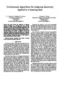
the frequency is represented on a logarithmic scale. Figure 1.3 shows the Bode diagram of a first order system expressed by G(s) = 1/(s + 1). The system behaves like a low-pass filter. It can be seen


17

as a RC circuit where the time constant τ = RC = 1. At low frequency the magnitude and the phase of the output are approximately the same as the input. At high frequency the magnitude of the output is attenuated and the phase presents a certain delay. Bode Diagram

Magnitude (dB)

0

−10

System: sys Frequency (rad/sec): 1 Magnitude (dB): −3.02

−20

−30

Phase (deg)

−40 0

−45

−90 −2 10

−1

10

0

10

1

10

2

10

Frequency (rad/sec)

Figure 1.3: Bode diagram for a first order system.

1.6.5

PID control systems: introduction and representation

A general closed loop controller (figure 1.1) implements the control variable u(t) as a function of the error e(t). A PID controller bases its action on the sum of three values derived from the error: a proportional action, a derivative action and an integral action. The weights of the three different actions are the parameters of a PID controller. The tuning of a PID controller consists in the search of the parameters that can optimize a pre-specified performance index within some particular constraints. The typology of PID controller is widely spread in industry where more than 90% of all control loops are PID (˚ Aström, Hägglund 2001). The action taken by a PID controller on the plant can be expressed in the time domain as

18

Introduction

µ ¶ Z 1 t de(t) u(t) = K e(t) + e(τ )dτ + Td Ti 0 dt

(1.7)

In the frequency domain, a PID controller can be expressed by the transfer function ´ ³ 1 + sTd GP ID (s) = K 1 + sTi

(1.8)

Equation (1.8) is called standard or non-interacting form (˚ Aström, Hägglund 1995). Equation (1.8) can also be written to highlight the three PID parameters as

GP ID (s) =

K3 s2 + K1 s + K2 s

(1.9)

where K1 , K2 and K3 are the weights of the proportional, integral and derivative actions. An alternative representation is expressed by ³ 1 ´ G0P ID (s) = K 0 1 + (1 + sTd0 ) sTi0

(1.10)

and is called serial or interacting form. The reason is that the controller (1.8) has the components assembled with a parallel structure. Thus, the proportional, integral and derivative actions do not influence each other. In the interacting controller (1.10), the derivative action influences the proportional and integrative actions through a serial connection. Every interacting representation has an equivalent non-interacting representation, but not vice versa. For this reason the non-interacting form is considered more general (˚ Aström, Hägglund 1995). The controllers used in this work are implemented with a non-interacting model form.

1.7

Criteria of Performance Evaluation

The problem of the evaluation of a control system performance has always been a central topic in control system theory. Constraints and requirements play an important role in the design of a controller.

1.7 Criteria of Performance Evaluation

19

With the emergence of evolutionary algorithms in control system engineering, the problem of the performance has become related to the evaluation of the fitness of a solution. For each control system, a performance index should be calculated in order to express the quality of the controller as a unique positive value. Often a performance index can become a constraint in the design of the system. Usually a performance index is a value that should be minimized in order to obtain a well tuned controller with good performance. A constraint is a performance index that should have values within a certain range and should not necessarily be minimized or maximized. In (Dorf, Bishop 2001) the following definition of performance index is given A performance index is a quantitative measure of the performance of a system and is chosen so that emphasis is given to the important system specification. The definition is generic because for different systems there might be different desired characteristics. For some systems, a very fast response could be the desired target in spite of an abrupt jump of the output variable. For other systems the movement of the output variable should be as smooth as possible paying the prize of a slower response. Performance indices and requirements are expressed in the time domain or in the frequency domain.

1.7.1

Time domain indices

Several indices are proposed. I will limit the description to the indices used in this paper. A measure of the difference between the reference value and the actual plant output, intended as the area between the two curves, is given by the IAE and ITAE indices defined as follows. The Integral of Absolute Error is expressed by Z

T

IAE =

|e(t)|dt.

(1.11)

0

The Integral of Time-weighted Absolute Error is expressed by Z ITAE =

T

t|e(t)|dt. 0

(1.12)

20

Introduction

Additionally, the Integral of Squared Time-weighted Absolute Error is expressed by Z IT2AE =

T

t2 |e(t)|dt.

(1.13)

0

where T is an arbitrarily chosen value of time so that the integral reaches a steady-state value. A system is considered optimal with respect of one performance index when the parameters are tuned so that the index reaches a minimum (or maximum) value. Equation (1.12) expresses a measure of the value of the error between the plant output Y (s) and the reference signal Yref (s) weighted on time. That means that the index penalizes more heavily errors that occur later. In setting the requirements for a controlled system, however, the IAE and ITAE performance indices provide a poor description of the system dynamics. Other values can better describe the characteristics of the response to a step reference signal or disturbance. Values commonly used in the specification and verification of a controlled systems are rise time, overshoot, settling time, delay time, steady-state error. Given a step input to the reference signal, which is intended to bring the output value from a value of Y1 to Y2 , we have the following definitions. - The delay time is the time taken by the system output to reach 50% of Y2 -Y1 . - The rise time is the time taken by the output to rise from 10% to 90% of Y2 -Y1 . Sometimes it is considered the rise time calculated from 0% to 100% of the step magnitude. - The overshoot is the amount the system output response proceeds beyond the desired value (Y2 ). The system is also said to ring when after the first peak, the output goes back under the reference signal of a certain percentage. - The settling time is the time required for the system output to settle within a certain percentage of the input amplitude. - The steady-state error e∞ is the error when the time period is large and the transient response has decayed leaving the continuous response.


1.7.2

21

Frequency domain indices

Performance indices or system specifications can be given in the frequency domain. A frequency domain approach to the design of control systems is also often used. Like in the time domain, the distinction between performance indices, characteristics and system specifications is blurred. An introduction to the frequency domain approach is far beyond the aim of this paper; I will limit myself to the description of few indices and evaluation criteria. The bandwidth of a system is defined as the frequency range 0 ≤ ω ≤ ωb in which the magnitude of the closed loop does not drop −3dB from the low frequency value. “The bandwidth indicates the frequency where the gain starts to fall off from its low-frequency value” (Ogata 1997). From equation √ (1.6), a value of −3dB is equivalent to an attenuation of the signal of 2/2 in the linear scale. The bandwidth gives an indication of how fast the system response is following a variation of the reference signal. A high bandwidth has the downside to amplify the noise present in the feedback line. Noise suppression requirements are often given in the frequency domain. A noise measured on the feedback is characterized by a range of frequencies and intensities. Feedback noise is often characterized by high frequencies. A desired characteristic of the control system is a pre-specified attenuation of frequencies above a certain value. Other important indices used in the frequency domain design are the gain margin and the phase margin. The gain margin is defined as the change in the open loop gain required to make a closed loop system unstable. The phase margin is defined as the change in open loop phase shift required to make a closed loop system unstable. For robustness reasons, a system is often designed with a minimum phase margin and gain margin.

1.7.3

Control constraints and requirements

When designing the controller and trying to optimize the chosen performance indices, particular attention should be devoted to the respect of the constraints. Each control problem has some kind of constraints due to physical or technological limitations, power consumption, etc. Constraints are often particular performance indices which describe a characteristic of the plant that should be maintained within a given range of values. The most significant constraints are described in the following list. 1. Overshoot ≤ OM AX Typical values of OM AX are 0%, 2%, 10%. By instance, the controller

22

Introduction

of an elevator should have OM AX = 0% since we want to avoid that the elevator goes a bit beyond the floor and then back to the desired level. In other situation, in order to obtain a faster movement, a value of overshoot within a certain percentage can be tolerated. 2. |u(t)| ≤ uM AX The value of the control variable u(t) is limited between −uM AX and uM AX . This is due to the limit of the actuator or the limit of the maximum strength applicable on the plant without causing damage. For example, the electrical engine of an elevator can apply a variable lifting power which has an upper limit due to the engine’s characteristic. A limit could also be imposed by the strength of the steel wire that can undergo a maximum tension. Finally, a limited lifting power may be required in order to assure a comfortable service to the users. 0

3. |u(t)| ˙ ≤ uM AX The varying rate of the control variable is limited by the characteristic of the actuator. Using the previous example of the elevator, suppose that the target is to move the elevator as fast as possible from one floor to an other using instantly the maximum power uM AX of the engine. The internal mechanical dynamics of the engine does not allow the control variable u(t) representing the applied power to go from 0 to uM AX instantly. Electrical engines however can reach the maximum power in a very short time. Contrary, if the system is a room to be warmed up and the control variable is the temperature of an electric heater, it is clear that some time is required before the heater reaches its maximum temperature and the control variable its maximum value. The same can be said for electro-mechanic valves, rudders, flaps and other mechanical parts in vehicles. The internal dynamic of the actuator should be carefully considered. Only after a precise study of the physics of the actuator, it is possible to decide to ignore it or not in the system model. 4. Saturated control allowed/not allowed For most of the industrial processes, the control variable should never reach the maximum value of saturation, or if it happens, for a very short time. Several reasons justify this constraint. One is the fact that most actuators require a very high power consumption to work at top revs. Besides, the effect of wear and tear increases enormously when an actuator is working at the limit of its capability. The nonlinear behaviour of the controlled system caused by the saturation is also often


23

undesired and u(t) ˙ presents a discontinuity when the saturation level is reached or left. Finally, when the control variable is saturated, the feedback loop is broken and the control system is not able to suppress load disturbance in this phase. Such kind of control is called bang-bang control, and it is suitable only for particular control problem. 5. |e∞ | ≤ eM AX For most of the control system a steady-state error of 0 is desired in order to make the output variable get indefinitely close to the reference signal during a steady-state condition of the system. A null steadystate error is obtained using an integral action in the controller. 6. Settling time ≤ target settling time A short settling time is often desired. However, a too low settling time constraint might result in an impossible solution due to the con0 flict with other constraints as uM AX or uM AX . If the settling time constraint is extremely important, the problem can be modified, in 0 order to obtain a possible solution, relaxing uM AX or uM AX . This is done using an actuator with better performance in terms of power and response. In some cases, economical or technological reasons hinder ambitious targets and a compromise on the settling time has to be chosen. 7. ωb ≥ ΩM IN This constraint is often used alternatively to the settling time constraint when designing the system using the frequency domain approach. In fact, the bandwidth of the closed loop system gives an indication of the reactivity of the system. Besides, a high bandwidth allows a good compensation of the disturbance at the plant input. A lower limit to the bandwidth is imposed when a disturbance of a given intensity at the plant input has to be suppressed. The higher the bandwidth, the better is the load disturbance suppression. A high band0 width constraint might be in contrast with uM AX or uM AX . Besides, the bandwidth has an upper limit imposed by the next constraint. 8. ωb ≤ ΩM AX This constraint is imposed to limit the bandwidth of the closed loop. A too high bandwidth amplifies the noise on the feedback bringing the control system to poor performance. Eventually the system can become unstable or the plant be damaged. Thus, this constraint should be set after a careful consideration of the level of noise present on the feedback signal. It is clear that ΩM IN has to be less than ΩM AX in

24

Introduction

order to make the design possible. When ΩM IN ¿ ΩM AX , ωb can be chosen in a large range. If the two limits are close, because load and feedback noise have close frequency, the design becomes more difficult. Other constraints used in the frequency domain design approach are the gain margin and the phase margin. The optimization of a performance index within the constraints that might be set for a specific control problem is equivalent to find the solution of an optimization problem. The search space is a hyperspace delimited by the hyper-planes corresponding to the constraints. The number of constraints that can be imposed by technological or environmental reasons suggests that, to design a good control system, a complete set of data should be obtained from the system to be controlled. In most of the cases measurements in situ of the noise intensity are necessary. That means, as pointed out in (˚ Aström, Hägglund 1995), that a deep understanding of the physics behind the process is necessary in order to design a good controller, understand which phenomena should be included in the mathematical model and which phenomena can be approximated or ignored.

Chapter 2

Problem Definition and Methods 2.1

The Control Problem

Dorf, Bishop (2001, example 12.9, p. 699) propose a design method for a robust PID-controlled system. The plant to be controlled is expressed by the transfer function

G(s) =

K (τ s + 1)2

(2.1)

For a robust system design, the two parameters K and τ are variable in the intervals 1 ≤ K ≤ 2 and 0.5 ≤ τ ≤ 1. The second order system of equation (2.1) is representative of several physical systems such as the mass-spring system, the temperature of a close environment and with some approximation the steering dynamics of a cargo ship. In the analysis, only the mathematical model is considered without addressing a specific physical system.

2.2

The Dorf, Bishop PID Controller

The controller described in (Dorf, Bishop 2001, page 697) is supposed to control a temperature. The performance index to be minimized is the ITAE index expressed by equation (1.12). The constraints are an overshoot less than 4% and a settling time less than 2 seconds. Several other constraints 0 like uM AX , uM AX and ΩM AX are implicitly considered and discernible from

26

Problem Definition and Methods

s + ωn s2 + 1.4ωn s + ωn2 s3 + 1.75ωn s2 + 2.15ωn2 + ωn3 s4 + 2.1ωn s3 + 3.4ωn2 s2 + ωn3 s + ωn4 s5 + 2.8ωn s4 + 5.0ωn2 s3 + ωn3 s2 + ωn4 s + ωn5 s6 + 3.25ωn s5 + 6.60ωn2 s4 + ωn3 s3 + ωn4 s2 + ωn5 s + ωn6 Table 2.1: Optimum coefficients of T(s) based on the ITAE criterion for a step reference signal. the final system. Other constraints like the noise suppression on the feedback are simply not mentioned. The problem is not completely specified and the controller is not completely described: it is important to notice that the purpose of the exercise in (Dorf, Bishop 2001, page 697) is to show a tuning method that is far from the implementation of a real and complete control system. In other words, the method explain how to tune the PID parameters in order to minimize the ITAE index and gives an extremely simplified example of a controller implementation. Thus, the results that can be obtained from the simulation of the system are qualitative and do not provide the performance of a real plant.

2.2.1

Method of Synthesis

For a general closed-loop transfer function as T (s) =

b0 Y (s) = n R(s) s + bn−1 sn−1 + · · · + b1 s + b0

(2.2)

Dorf, Bishop (2001, p. 252) give the coefficients (table 2.1) that minimize the ITAE performance criterion for a step reference signal. The value of ωn (the parameter of the equations in table 2.1) will be limited by considering the maximum allowable u(t), where u(t) is the output of the controller. Table 2.2 shows the effect of ωn on the intensity of the control variable and settling time (Dorf, Bishop 2001). ωn u(t) maximum for R(s) = 1/s Settling time (sec)

10 35 0.9

20 135 0.5

40 550 0.3

Table 2.2: Maximum value of plant input given ωb

2.2 The Dorf, Bishop PID Controller

27

A generic PID controller is expressed as Gc (s) =

K3 s2 + K1 s + K2 . s

(2.3)

Hence, the transfer function of the system (for K = 1, τ = 1) without pre-filtering is1

T1 (s) = =

Y (s) Gc G(s) = = Ysp (s) 1 + Gc G(s) K3 s2 + K1 s + K2 s3 + (2 + K3 )s2 + (1 + K1 )s + K2

(2.4)

From equation (2.4) and table 2.1 K3 = 1.75ωn − 2 K1 = 2.15ωn2 − 1 K2 = ωn3

(2.5)

From the parameters (2.5) and equation (2.3), the transfer function of the compensator is

Gc (s) =

12 · (s2 + 11.38s + 42.67) s

(2.6)

Finally the equation of the pre-filter

Gp (s) =

s2

42.67 + 11.38s + 42.67

(2.7)

is obtained so that the overall transfer function has the same form of equation (2.2). The overall controlled system is expressed by the transfer function Y (s) 512 = T (s) = 3 R(s) s + 14s2 + 137.6s + 512 1

(2.8)

A closed loop transfer function G(s) is related to the open loop transfer function L(s) L(s) by the relation G(s) = 1+L(s) .

28


Equation (2.8) shows T (s) for the values of the parameters K = 1, τ = 1. The system can be specified by a Matlab script that, given the parameter K and τ , calculates the transfer function T(s). Appendix ± A.5 reports the script used for the purpose. T (s) is expressed as N (s) D(s) where N (s) and D(s) are vectors representing the numerator and denumerator of the transfer function. An alternative way to represent and simulate a PID controlled system is using Simulink.

2.3

The GP controller

The target of the design process in (Koza et al. 2003) is more ambitious. The genetic computation evolved a controller by means of a simulation-based fitness calculation. The target is not the description of a tuning system, but the real design of a complete controller, from the structure to the choice of the parameters. The constraints imposed for the simulation are (Koza et al. 2003, col. 47) • Overshoot: Omax ≤ 2% • Control variable: |u(t)| ≤ uM AX = 40V olts. • Limited bandwidth for the closed loop Y /Yref . “The second constraint is that the closed loop frequency response of the system is below a 40dB per decade low-pass curve whose corner is at 100Hz”. (Koza et al. 2003, col. 47). That means that the maximum bandwidth allowed ΩM AX is 401rad/sec and after this value the attenuation is 40dB per decade2 . In (Koza et al. 2003) it is also said that “This bandwidth limitation reflects the desirability of limiting the effect of high frequency noise in the reference input”. From this list of constraints, some important observations have to be made. The bandwidth of the closed loop from the reference signal Yref to the plant output (Y /Yref ) is different from the bandwidth of the closed loop from the filtered signal to the output (Y /Yf il ). This is due to the presence of a pre-filter between the reference signal and the point of the error calculation. If we consider figure 1.1 the two transfer functions just mentioned are the 2

Using the conversion 1Hz = 6.28rad/sec, the reference low-pass filter transfer function 6282 is expressed by G(s) = (s+628) 2

2.3 The GP controller

29

same function. A limit on the bandwidth does not only limit the noise at the reference signal, but even the noise on the feedback signal, because the point of application is the same. If we now consider figure 1.2, when a pre-filter is introduced, the point where the reference signal is applied differs from the point where a feedback noise is applied. As a consequence, the limitation of the bandwidth for Y /Yf il becomes largely independent from the limitation of the bandwidth on the reference signal. That means that the constraint regarding the bandwidth limit for the closed loop Y (s)/Yf il (s) is missing. The consequence is that the bandwidth can be as high as desired and the load disturbance can be suppressed up to any desired level. Thus, even before the simulation we can draw a hypothesis on the 9 times better performance claimed for the GP in (Koza et al. 2003). On the other hand, this implies the necessity of a feedback signal free of noise. Unfortunately, as a matter of fact, there is not any physical measurement tha can be considered free of noise or uncertainty. This makes any controller designed without a limit constraint on the bandwidth a theoretical controller without chances to be implemented. The reason why the GP controller shows a disturbance attenuation only 9 times better than the PID is probably due to quantization and sampling noise: the digital simulation of an analog system, however precise, implies a numerical approximation which eventually can be seen as noise in the signal (Haykin 2001). Another important constraint missing is the maximum value of u(t). ˙ This is possible where the dynamics of the actuator is extremely fast in comparison to the dynamic of the system. In these cases u(t) ˙ can vary up to any extremely large value.

2.3.1

Linear Representation

In (Koza et al. 2003) the plant to be controlled is the one just described in section 2.1. The authors of the invention have chosen that plant on purpose to be able to compare their GP controller to the textbook controller. The proposed pre-filter is3 3

The equation is reported modified as in (Soltoggio 2003) according to the presumed printing errors found in the original paper (Koza et al. 2003).

30


Gp (s) = =

1(1 + 0.1262s)(1 + 0.2029s) (1 + 0.03851s)(1 + 0.05146s)(1 + 0.08375s)(1 + 0.1561s)(1 + 0.1680s) (2.9)

In order to emphasize the gain and the zeros/poles values, the transfer function (2.9) can be rewritten as follows Gp (s) = =

5883.01 · (s + 7.9239)(s + 4.9285) (s + 25.9673)(s + 19.4326)(s + 11.9403)(s + 6.4061)(s + 5.9524) (2.10)

The transfer function for the proposed compensator is 7497.05 + 1300.63s + 71.2511s2 + 1.2426s3 (2.11) s The values of the numerator of the previous function correspond to the integral, proportional, derivative and second derivative actions. The Matlab script reported in section A.6 is used to calculate, from equation (2.9), (2.11) and the values for K and τ , the transfer functions Y (s)/Ysp (s) and Y (s)/Df (s). Gc (s) =

2.4

The GA controller

The GA controller makes use of the same constraints of the GP controller plus an additional constraint. The derivative of the control variable, u(t), ˙ was limited to 10,000 Volts/sec. Although this is a high value, the limitation is determinant to constrain the GA search. In fact, preliminary runs showed that the search process is apt to exploit an unlimited u(t) ˙ to reach a very high load disturbance suppression until quantization and sampling noise arises and acts as a hidden constraint. The complete and detailed description of the GA controller and method is given in chapters 4 and 5.

2.5

Implementation of the Derivative Function

The transfer function of a derivative is often expressed as G(s) = s, as defined with equation (1.2) and used in the previous sections. This is an

2.5 Implementation of the Derivative Function

31

approximation and improper use of the concept of transfer function. In fact, a transfer function can not have more zeros than poles, i.e. the grade of the denominator must be superior to the the grade of the numerator. This is due to the impossibility for the output to predict the future signal to the input. Thus, the mathematical operator s is used as an approximation of the real function

G(s) =

s . τd s + 1

(2.12)

In some text books a PID controller is expressed directly using equation (2.12) (Nachtigal 1990). Equation (2.12) can be written as the series of a derivative and a low-pass filter

G(s) = s ·

1 τd s + 1

(2.13)

When the time constant τd of the low pass filter is very small in comparison to the time constant of the process, the function (2.12) can be considered a good approximation of a derivative function for frequencies below τ −1 rad/sec (Nachtigal 1990). The choice of τd is the result of an accurate compromise: a very small τd implies a large bandwidth for the low-pass filter and gives a very good derivative function with a small loss in phase margin. It has the downside to be very sensitive to noise, though. For this reason, this approach is actually used very seldom. Increasing the value of τd gives a narrower bandwidth with the capability of suppressing high frequency noise. The downside is that the phase margin decreases and so the accuracy of the derivative. Eventually, a too narrow low-pass filter would decrease the phase margin to a dangerous level of the stability threshold. Figure 2.1 shows the effect on the stability of the system when a too narrow low-pass filter is applied (τd = 10−1 ). A further increment of τd makes the system unstable with oscillations that are getting wider with time: for this reason a robust controlled system is often designed with a minimum phase margin requirement. Both the analysed systems are supposed to be free of noise on the feedback (see section 1.7.3). For this reason there is no need to implement a narrow low-pass filter. However, the numerical simulation of a continuous system implies digital approximation. This has the very same effect of noise. The derivative and especially the double derivative of the GP controller feel

32


1

Plant Output (Volts)

0.8

0.6

0.4

0.2

0

0

0.2

0.4

0.6 Time (sec)

0.8

1

1.2

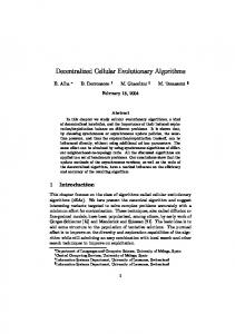
Figure 2.1: Effect on the plant output of a too narrow low-pass filter on the derivative the effect of such noise. Figure 2.2 shows the effect on the derivative control variable when τd = 10−4 . A derivative operation applied on signal of figure 2.2, as in the case of the GP controller, is simply not feasible. A solution to the problem can be found increasing the sampling of the simulation or using a stiff solver as ode15s(stiff/NDF). Yet, this effort does not help to make the simulation realistic: in real problems the feedback signal is affected by disturbance. For this reason, while implementing the controller, the intensity and characteristic of the noise have to be taken into account. Given the specification of free-of-noise feedback signal and therefore the requirement for an accurate derivative function combined with the necessity of filtering the numerical approximation, I chose the following compromise: I implemented the derivative function as

Gd (s) =

τd−1 s s + τd−1

(2.14)

where τd−1 = 1000. This value gives a good approximation of a derivative function4 and it is not affected by the numerical approximation. Figure 2.3 4

A simulation of a controller with a double derivative has provided a very accurate

2.6 The MathWorks Inc. Software

33

60

Derivative variable intensity (Volts)

50

40

30

20

10

0

−10

0

0.2

0.4

0.6 Time (sec)

0.8

1

1.2

Figure 2.2: Effect on the control variable of a too relaxed low pass filter on the derivative. Sampling step: 0.001sec; Solver: ode45(Dormand − P rince) shows the Bode and phase diagram of equation (2.14). The diagram shows that the function is a good approximation of a derivative for frequencies up to 103 rad/sec. Simulink offers a derivative block du/dt which is intended to provide the derivative of the input at the output. During the simulation of both the models with the derivative blocks, I encountered the same simulation problems described above due to numerical approximation behaving like noise. For the derivative block, unlike for other blocks, the solver does not take smaller steps when the input changes rapidly (The MathWorks Inc. 2002, p. 2-69). The simulation was only possible with a stiff resolution method (ode15s) and produced in some cases wrong results.

2.6

The MathWorks Inc. Software

The application used for the experiments reported in this thesis is coded entirely in the Matlab environment. The reason to use Matlab is the importance and complexity of the fitness evaluation for the present optimization problem. The control system to be simulated and evaluated is run by the Simulink second derivative function with zero values few µseconds delayed from the peak of the first derivative.

34


Bode Diagram

60

Magnitude (dB)

50 40 30 20 10

Phase (deg)

0 90

60

30

0 1 10

2

10

3

10

4

10

5

10

Frequency (rad/sec)

Figure 2.3: Bode and phase diagram for the derivative plus low-pass filter transfer function of equation (2.14)

engine. Simulink is called during each generation to evaluated each individual of the population and returns a time domain vector of the system output and the control variable. From this data an m file compute the fitness. After all the individuals are evaluated, an m file produce a new generation and other m file carries out the main GA cycle and plot the partial result of the computation. Using Matlab, it was possible to code the whole application in the same environment and utilize both the functionalities of Matlab and Simulink for the genetic algorithm and the fitness evaluation respectively.

Chapter 3

A Genetic Programming Approach 3.1

Description

The method for the automatic synthesis of controllers proposed in (Koza et al. 2000) and fully explained in a United States Patent (Koza et al. 2003) consists in a complex setting of software, machines and choices of parameters. Given a description of the plant and the constraints of a control problem, the purpose of the method is the automatic generation of a controller that constitutes a solution to the problem. The reference documents used in this paper have the purpose to explain in details the invention proposed. Here the description will be limited to a brief overview. The two-lag controller studied in this paper was created using a parallel computer architecture of 66 computers. Each computer contained a 533MHz DEC Alpha microprocessor and 64 megabytes RAM. The computers were connected with a 100 megabit/sec Ethernet. The processors and the host used the Linux operating system. The method makes use of a genetic programming technique (Koza 1992) (Banzhaf et al. 1998). The program tree represents the block diagram of a controller. In this embodiment, the program tree is converted into a phenotype represented by a SPICE netlist. The controller is therefore implemented as an electronic circuit. The program architecture trees make use of automatically defined functions (ADFs)1 . The architecture-altering operations may insert and 1

An ADF is a function whose body is dynamically evolved during the run and which may be invoked by the main result-producing branch(es) or by other automatically defined

36

A Genetic Programming Approach

delete ADFs to particular individual program trees in the population. The set of terminals identifies the input and output of the blocks represented in the program tree. Some of the terminals used are REFERENCE SIGNAL, PLANT OUTPUT and CONTROLLER OUTPUT. The repertoire of functions is wide and comprehends one or more argument functions; an example set of functions is provided below, a complete list of all the functions used by the method is provided in (Koza et al. 2000, pages 134, 135) and (Koza et al. 2003, col. 48). The one-argument INVERTER negates the time domain signal represented by its argument. The one-argument DIFFERENTIATOR differentiates the input signal and represent the transfer function s (see section 1.6.3). The one-argument INTEGRATOR represents the transfer function 1/s. The two argument LEAD function applies the transfer function 1 + τ s. The two-arguments LAG function applies the transfer function 1/(1 + τ s). The fitness is determined by a combination of different elements. Eight time domain based ITAE indices are calculated for different combinations of the plant parameters, as explained in section 2.1, and step reference signals. Two step reference signal of 1 Volts and 1µVolts are used. One time domain element measuring the stability when faced with an extreme spiked reference signal and one element represented by a frequency domain index are added. The values obtained by the different indices are added to obtain a single fitness value. The smaller the fitness, the better. The time domain analysis was carried out in an interval of time of 9.6 seconds. The ITAE index was used in the following modified form Z

t=9.6

t|e(t)|A(e(t))Bdt

(3.1)

t=0

where B represents the inverse of the step reference signal so that the 1Volts and 1µ Volts signal have the same weight. The function A weights all variations below the reference signal and up to 2% above the reference signal by a factor or 1.0 and heavily penalizes overshoots over 2% by a factor 10.0. A discrete approximation to the integral was used by considering 120 80-millisecond time steps in the interval 0 ≤ t ≤ 9.6 seconds. The control parameters for the run comprehend the population size, the maximum size of the program tree and the percentage of the different genetic operations applied. The population size was 66.000, each node having 1000 individuals. Generations are run asynchronous on each node. For each function(s) (Koza et al. 2000, page 136). More information about ADFs can be found in (Koza 1992), (Koza 1994) and (Banzhaf et al. 1998)

3.2 Simulation results

37

generation four boatloads of emigrants are dispatched to each of the four adjacent processing nodes. The boatloads have 20 emigrants chosen on a fitness basis. The maximum size of the program tree was 150 points and 100 points for each automatically defined function. The percentages for the genetic operations on each generation up to and including generation 5 were 78% one-offspring crossover, 10% reproductions, 1% mutations, 5% subroutine creations, 5% subroutine duplications and 1% subroutine deletions. After generation 5 the percentages were 86% one-offspring crossover, 10% reproductions, 1% mutations, 1% subroutine creations, 1% subroutine duplications and 1% subroutine deletions. The termination criterion was not set since the run was manually monitored and manually terminated when the fitness of many successive best-ofgeneration individuals appeared to have reached a plateau. Each individual of the population required an average of 4.8 seconds to be evaluated. The best individual from generation 32, which block diagram is represented in figure 3.1, was produced after evaluating 2.57 · 106 individuals (66,000 times 33). The necessary time for the computation was 44.5 hours with an expenditure of 5.6 · 1015 computer cycles.

3.2

Simulation results

The simulation of the GP controller, compared to the standard PID as fully described in (Soltoggio 2003), shows that the GP controller uses the control variable in a more intensive way than the PID. It makes use of saturated control and higher varying rate of the control variable. Figure 3.2 shows the control variable for both the controllers. The use of nonlinear, saturated control helps the GP controller to achieve a faster response. Besides, the GP controller as presented in (Koza et al. 2000, Koza et al. 2003), uses a second derivative that, without the introduction of a proper low-pass filter, produces a very high bandwidth. Moreover, the lack of a constraint for the derivative of the control variable and the unlimited bandwidth in the feedback loop (Y (s)/Yf eedback (s)) allows a potentially infinite load disturbance suppression but is not implementable on a real system. For the simulation, the derivative was implemented with an embedded first order low-pass filter in order to obtain a finite bandwidth as explained in section 2.5. The results of the simulation of the GP controller are reported in tables 3.1 and 3.2 where the GP controller is compared to the PID for K = 1, τ = 1 and K = 2, τ = 0.5.

r

Reference signal

Step

1

1 s 8.15

0.0385s+1

0.0837s+1 0.001s+1 TF4

0.001s+1

TF5

Gain1

Integrator Gain3 TF3

0.001s+1

Feedback

Control Variable

Saturation

Gain

-1

-1 Gain4

-1

0.0515s+1

TF2

0.156s+1

1

TF1

0.168s+1

GP Controller and Plant

cv2

Gain2

918.8

K

Load disturbance

PLANT

tau^2.s 2 +2*taus+1

Clock

y2 Plant Output

Time

t2

38 A Genetic Programming Approach

Figure 3.1: Simulink block diagram of the GP controller


39

40

K = 1, τ = 1 K = 2, τ = 0.5

GP control variable

Control Variable (Volts)

30 20 10 0 −10 −20 −30 −40 0

0.1

0.2

40

0.3 Time (sec)

0.4

0.6

K = 1, τ = 1 K = 2; τ = 0.5

PID control variable

30 Control variable (Volts)

0.5

20 10 0 −10 −20 −30 −40 0

0.1

0.2

0.3 Time (sec)

0.4

0.5

0.6

Figure 3.2: Control variables for the GP and the textbook PID controllers From the analysis, the controller presented in (Koza et al. 2000, Koza et al. 2003) has substantially different characteristics from the PID and is therefore not comparable. However, the design method explained in (Dorf, Bishop 2001, pages 697-700) allows to tune the PID control variable to any desired value. Hence, in a second simulation, the standard PID controller was tuned for a stronger control action tentatively setting the tuning parameter ω from 8 to 16; additionally, a limit on the integral was imposed to 8 Volts and a gain of 3 was added to the feedback signal. The roughly tuned controller, compared to the GP controller, obtained better performance under all the considered indices. Table 3.3 shows the simulation results for K= 1 and τ = 0.5. It was observed from the simulations that both the GP controller and the tuned PID bring the control variable to saturation for the plant parameters K = 1 and τ = 1; i.e. when the plant has the lowest gain (K) and the highest time constant (τ ) and needs a stronger control action. For the other 2

Overshoot is limited to 2% |u(t)| is limited to 40V olts 4 The bandwidth for Y /Ysp is limited to 401rad/sec 5 With the same limitations as above 3

40


Overshoot Delay time (ms) Rise time (ms) Settling time (ms) ITAE (mVolts · sec2 ) Load disturbance deviation (mVolts) IAE of disturbance (µ Volts · sec2 ) Maximum u(t) (Volts) Maximum u(t) ˙ (Volts/sec) Saturated control Actuator usage Bandwidth Y /Yref (rad/sec) Bandwidth Y /Yf eedback (rad/sec)

PID

GP

2% 261 290 943 48.6 6.4 197.0 24.6 495 No 11.24% 8.2 19.9

1.5% 174 181 300 18.5 0.670 22.0 40 3087 Yes 86.45% 9.6 51.7

Characteristic limited2 to minimize to minimize to minimize to minimize to minimize to minimize limited3 unspecified/free unspecified/free unspecified/free limited4 unspecified/free

Table 3.1: Summary of data for the PID and GP controller for K = 1, τ = 1

Overshoot Delay time (ms) Rise time (ms) Settling time (ms) ITAE (mVolts · sec2 ) Load disturbance deviation (mVolts) 2

IAE of disturbance (µ Volts · sec ) Maximum u(t) (Volts) Maximum u(t) ˙ (Volts/sec) Saturated control Actuator usage Bandwidth Y /Yref (rad/sec) Bandwidth Y /Yf eedback (rad/sec)

PID

GP

0.35% 241 407 661 49.9 5.8 316.4 4.65 430 No 1.27% 5.2 113

0.5% 154 243 419 20.0 0.631 26.7 9.8 2766 No 2.30% 8.6 4640

Characteristic5 limited to minimize to minimize to minimize to minimize to minimize to minimize limited unspecified/free unspecified/free unspecified/free limited unspecified/free

Table 3.2: Summary of data for the PID and GP controller for K = 2, τ = 0.5


Overshoot Rise time (ms) Settling time (ms) 2

ITAE (mVolts · sec ) Load disturbance deviation (mVolts) Maximum u(t) (Volts) Maximum u(t) ˙ (Volts/sec) Bandwidth Y /Yf eedback (rad/sec) Bandwidth Y /Yref (rad/sec)

41

(PID)

(GP)

(tuned PID)

Characteristic

0.3% 391 629 49.0 6.0

0.4% 239 417 19.8 0.64

1% 210 326 13.5 0.42

limited to 2%

8.6 460 57.6

19.4 1927 3070

36.0 8761 435

limited to 40Volts

5.4

8.8

10.4

limited to 401rad/sec in (Koza et al. 2003)

to minimize to minimize to minimize to minimize

unspecified/free unspecified/free

Table 3.3: Simulation results for the PID, GP and new PID controllers for K = 1, τ = 0.5 three combinations of the parameters, the system response does not change significantly and the control variable remains under the saturation limit: the controllers use saturated control only in one fourth of the cases. This observation gave the notion that performance in the time domain could be improved by using even stronger control within the constraints. The following GA was designed to explore this possibility.

3.2.1

Frequency analysis of the GP controller

Table 3.4 presents a frequency analysis of the GP controller. The behaviour of the GP controller is linear in three of the four combinations of parameters. The first line presents the values of the bandwidth from the reference signal to the output. The second line reports the bandwidth from the filtered reference signal to the output with the filters on the derivatives. The third line reports the bandwidth of the system as described in (Koza et al. 2003) without the addition of the filters on the derivatives. It is evident that without the addition of a filter on the second derivative, the system, as specified in (Koza et al. 2003), is not implementable because it presents an infinite bandwidth. With the addition of a filter, the bandwidth is however quite high if compared to the PID. The missing constraint on the bandwidth of the closed loop and the absence of noise allowed the EC to increase the bandwidth to obtain the highest disturbance suppression possible.

42


ωb Y /Ysp (rad/sec) ωb Y /Yf il (rad/sec) (modified) ωb Y /Yf il (rad/sec) as in (Koza et al. 2003)

K=1

K=1

K=2

K=2

τ =1

τ = 0.5

τ =1

τ = 0.5

9.6 51.76 ∞7

8.8 3070 ∞

9 1720 ∞

8.6 4640 ∞

Table 3.4: Bandwidth for the GP controller closed loops

6

However the frequency response does not go under −5.4dB before ω = 1000rad/sec. An attenuation of −3bB is reached for ω = 48.2rad/sec, yet the frequency response never goes under -5dB, that is equivalent to have an infinite bandwidth. 7

Chapter 4

A Genetic Algorithm Application 4.1

Motivations and Proposed Targets

The genetic programming approach for the synthesis of a controller for a second order linear plant requires intensive computation. Besides, the given problem is considered one of the simplest in control engineering. The reasons of the poor results obtained by (Koza et al. 2003, Koza et al. 2000) can be found in the fact that optimal structures and parameters tuning for a second order plant are well known by the traditional control engineering. Evolutionary computation is not likely to perform well when traditional methods offers optimal solutions. However, tuning techniques and controller structure settings become more complex when nonlinearities and noise are introduced in the system. The idea of using GAs for the synthesis of a controller in presence of nonlinearities such as saturation, rate limiter or dead zone, arises from the attempt of finding a compromise between the GP technique and the traditional method. In other words, GAs offer the opportunity of easily embedding controller structure requirements and restrict the search to a well defined space. Doing so, the complex fitness landscape that arises from nonlinearities and presence of noise can be tackled by evolutionary computation without being lost in the too wide search space of the GP method. The proposed target is the synthesis of a time optimal controller for the constrained linear control system (equation 2.1) with disturbance rejection.

44

A Genetic Algorithm Application

1 In1

K tau^2.s2+2*taus+1

1 Out1

PLANT

Figure 4.1: Single Simulink block for the simulation of the plant of equation 2.1 Preliminary experiments The development of the application was characterized by continuous experiments, which I define preliminary runs, in order to identify a proper parameter setting and understand the dynamics in the evolution of the population. Most of the expertise was acquired in this phase by the analysis of the initial flaws. Hence, from the preliminary runs, a certain amount of experimental data or evidence was acquired. The quantity of details that was learnt during the practical attempt to implement a GA is large and too scattered to be completely described in this thesis. The choice of not providing a detailed experimental evidence of all the implementation choices was made to efficiently focus on the central and most significant results of the work. As a consequence, in the following sections, I will justify particular implementation choices as results of preliminary runs without providing the experimental proof.

4.2 4.2.1

Identification of the Search Space Simulink Model of the Controlled System

The plant In developing an automatic search algorithm for control engineering, the identification of the controller structure and the search space is strictly connected to the problem identification and the setting of constraints and requirements. Therefore, a deep preliminary study of the given control problem is essential. The description of the physic of the plant is the first important operation to do in order to obtain a good model and accurate simulations. One of the weak points of EAs in control synthesis is the lack of mathematical proof of stability: the guarantee that the designed controller will work once applied in the real plant relies entirely on the fidelity of the simulation. The plant of equation (2.1) can be expressed by a single Simulink block as in figure 4.1.

4.2 Identification of the Search Space

45

However, the block of figure 4.1 does not specify the physical constraints of the plant. As explained in sections 1.6 and 1.7.3, a physical action is performed by an actuator that has a limited power and whose output has a limited power spectral density (PSD), i.e. limited varying rate. The automatic mechanism of synthesis implemented by means of EAs has to be constrained with elements that in the traditional design are often omitted. In (Dorf, Bishop 2001, pages 697-700), saturation and rate limit are not considered because the design takes for granted that high performance cannot be reached using indefinitely high control action and indefinitely high varying rate. For the plant of equation (2.1), the response to a step reference signal can be made as fast as desired by using an arbitrary high value of the control variable. In particular, for a control variable and a varying rate approaching infinity, the rising time, settling time, ITAE and error approach zero. What seems to be obvious using the common sense, has to be strictly specified and constrained in an EAs application. Hence, the plant represented in figure 4.1, can be better specified as in figure 4.2, where In1 is the control variable, In2 the load disturbance, Out1 the plant output and Out2 the actual control action performed by the actuator. cv

1 Out2

Control Variable 1 In1

K tau^2.s2+2*taus+1 Saturation Rate Limiter

2 Out1

PLANT 2 In2

Figure 4.2: Simulink model for the simulation of a constrained version of the plant of equation 2.1

The Controller Figure 4.3 shows the complete controlled system model as used in (Soltoggio 2004b). The model is composed by several parts having different functions. The error calculation is done after pre-filtering a step reference signal by means of the block called “Pre Filter”. The setting of this block is done by tuning three parameters: N1, D1, D2. Since the tuning of the pre-filter is done independently from the tuning of the PID parameters, a controller with this structure is called a two-degree of freedom controller.

46


The step reference signal can be substituted by other shapes of reference signal such as ramp or sine wave. The error feeds the PID core. The proportional part is simply represented by a gain (Kp). The integral part is achieved by means of a standard anti windup structure as described in (Bolzern et al. 1998, pages 423-427). The derivative part is implemented, as explained in Section 2.5, by using a first order lowpass filter with a pole at the frequency of 1000rad/sec. The PID core is implemented using a non-interacting structure (see section 1.6.5). The three PID actions are summed to form the control variable at the input of the plant. The second input of the plant (In2) receives a load disturbance generated by the “Pulse Generator 2”. Alternatively, a load disturbance can be represented by a white noise, a sine wave or the combination of more signals. The plant output is fetched by an ideal sensor with transfer function equal to 1 and for this reason not represented in the diagram. The sensor introduces a high frequency noise generated by the block identified as “Noise on the feedback”. The noise can be applied for a limited amount of time by multiplying it with a pulse generator. Finally, the feedback signal is passed through a low-pass filter implemented with a Butterworth filter provided in the Simulink library. The filter is set in the panel shown in figure 4.4. The feedback gain (Kf) has the function of increasing or decreasing the bandwidth of the closed loop. Search Space Given the structure just described, the search space was defined by the following ranges of values N1 = [0,2000]; Kp = [0,2000]; Kf = [0,100]; Bw = [0,4000];

D1 = [0,2000]; Ki = [0,3000]; DerFac = [0,4000]; Ord = [1,8].

D2 = [0,2000]; Kd = [0,1000];

High pass filter for the feedback noise The noise that can affect the feedback signal can have low, high or both low and high frequencies. When the feedback signal is affected by a low frequency noise, there is no other solution than adding multiple sensors to correct the error (˚ Astr¨ om, Hägglund 1995). Contrary, for high frequency feedback noise, a low pass filter or a specified limitation on the closed loop bandwidth of the system can filter the noise and obtain a clean signal. The Band-Limited White Noise block, included in the Simulink library, produces both high and low frequencies.

Step

Clock

Kf*N1

Time

time

Pre Filter

D1.s2+D2.s+N1

Feedback gain1

Kf

Derivative gain

Kd

Proportional gain

Kp

Ki

Derivative

s+DerFac

DerFac.s

s+1000 Integrator - Anti wind up

_

Analog Filter Design

butter

Pulse Generator2

In2

In1

Product

Plant

Out1

Out2

Pulse Generator1

Noise on the feedback

Plant Output

output

4.2 Identification of the Search Space 47

Figure 4.3: Simulink model of the complete controlled system

48


Figure 4.4: Butterworth control panel in Simulink The power spectral density (PSD) of such a signal with sampling time 1ms and power 10−9 W is shown in figure 4.5. The effect of low frequency noise are evident on the control variable that oscillates to follow the low frequency noise. This behaviour is not so harmful as high frequency noise, however, it will affect the Integral of Absolute Error between the control variable and its steady state value (given by the inverse of the plant gain). Since the effect of noise on the feedback is measured through the IAE of the control variable, a certain amount of IAE will remain during steady state even in front of optimal filtering. To avoid this problem, in addition to the design in (Soltoggio 2004b), a high pass filter is introduced as shown in figure 4.6. The Butterworth block is set with passband edge at 800rad/sec and filter order equal to 3. The output of the high pass filter has low frequencies considerably attenuated as shown by the correspondent plot of the PSD shown in figure 4.7.

4.2.2

Solutions for Generation Zero and Randomized Seeds

A major problem in the GA search process is the initialization of the population. Preliminary runs showed that the quality of the seeds highly affect the search speed and in some cases, the quality of the results as well. To initialize the population, different approaches can be used as explained below.

4.2 Identification of the Search Space

49

−56

Power Spectrum Magnitude (dB)

−57

−58

−59

−60

−61

−62

−63

−64 0

0.1

0.2

0.3

0.4

0.5 0.6 Frequency

0.7

0.8

0.9

1

Figure 4.5: Power spectral density of the signal generated by the BandLimited White Noise block

butter

Noise on the feedback Analog Filter Design1

Figure 4.6: Generation of high frequency feedback noise 1. Initialization of the population with random values uniformly distributed in the search space. 2. Initialization as in the previous point with the insertion of well performing seeds obtained with other methods. 3. Initialization with random values whose expected value represent one or more seeds. This is done by randomizing seeds through normal or Gaussian distribution. The technique of point 1 is the most traditional in GA. Once the search space has been defined, the population is easily generated without application of further knowledge. The main problem is that when the search space is large and the population relatively small, the search process be-

50


−50

Power Spectrum Magnitude (dB)

−55

−60

−65

−70

−75 0

0.1

0.2

0.3

0.4

0.5 0.6 Frequency

0.7

0.8

0.9

1

Figure 4.7: Power spectral density of the signal produced by the BandLimited White Noise block and a Butterworth high pass filter come slow and the result is uncertain. This is particularly true when the fitness landscape is ill-behaved. The technique of point 2 allows a faster search thanks to the initial insertion of solution with good fitness. The approach has a main flaw though. For large search spaces as the one proposed in the previous section, the seeds during generation zero perform much better than the random generated individuals. During the following generations, it is likely that the offsprings of the seeds take over in the population and bring to extinction all the random solutions. This might not be completely true since some genes of the random solutions can survive if passed by crossover. However, the early extinction of the random generated solutions could suggest that to start with a population entirely seeded with good solutions is a better approach. This idea has a drawback as well. In fact, unless we are able to generate a number of different seeds equivalent to the cardinality of the population, we have to place two or more identical individuals in the population. As a limit, if we have only one seed, all the individuals are identical and the initial population is localized in a single point in the search space. If this point is the only good point known and it is clear that random points perform very badly in comparison and do not have any chance to survive, this approach can be a good choice. Yet, a population formed by identical individuals brings zero diversity and totally inhibits the operation of crossover. This situation persists until mutation introduces enough diversity in the population to

4.3 Fitness Composition

51

make crossover effective. The third approach was introduced in the attempt of finding a compromise between the first and the second method. It allows to maintain, to a certain degree, the quality of the seeds and introduce a certain amount of population diversity to enhance the crossover operation. The idea is to seed the population with one or more repeated seeds and randomizing them by multiplying each parameter of each individual by a random number with normal or Gaussian distribution. A variance vector represents the uncertainty assigned to a specific gene. Formally, for a n-dimensional genotype where −−−→ seedj =< s1 , s2 . . . sn > ,

(4.1)

− −→ =< σ 2 , σ 2 . . . σ 2 > , var j 1 2 n

(4.2)

and

we can write that −−−−−→ indivj,0 =< s1 · U (1, σ12 ), . . . sn · U (1, σn2 ) >

.

(4.3)

This is practically implemented using a vector of weights w =< w1 , . . . wn > that represents the variance and −−−−−→ indivj,0 =< s1 + s1 · w1 · U (1, σ 2 ), . . . sn + sn · wn · U (1, σ 2 )) .

(4.4)

The variance, defined through the weights, determines the strength of the randomizing process for each gene; the higher the variance, the higher the diversity in the population. If a weight is equal to 0, it means that the specific gene is not affected by uncertainty. If all the weights are set to 0, the seeds are left unmodified. A high value of the weights produce high variance and a gene might be assigned a value outside the search space. In this case, the value is assigned the maximum or the minimum allowed value.

4.3

Fitness Composition

The task of capturing a controlled system performance and returning a unique value describing the quality of a solution was one of the most difficult of this work. Several indices are considered with different purposes.

52


1. Integral of the Time-weighted Absolute Error (ITAE) between the reference signal and the actual output as expressed by equation (1.12) 2. Integral of the Squared Time-weighted Absolute Error (IT2AE) between the reference signal and the actual output as expressed by equation (1.13). 3. Exceeding overshoot 4. Exceeding ring 5. Exceeding zero crossings 6. Integral of Absolute Error between the control variable and its steady state value. The first two indices express the rapidity of the response. Overshoot and ring imply a penalty when the signal exceed ±2% the reference signal. Zero crossing is the number of zero crossings of the control variable. A limited amount is desirable to avoid instability of the control variable. The IAE of the control variable is used as further verification that the control variable does not undergo oscillations. The simulation time was set to be three times the settling time of the best individual. A first part of the simulation time corresponding to 2/3 of the total time was considered reserved to the transient. In the second part, from 2/3 to the end, the system was considered at steady state. Figure 4.8 helps to understand the division with a system showing a correct behaviour. The ITAE and IT2AE were calculated for all the simulation time, as well as Overshoot, Ring and Zero crossings. The IAE of the control variable was calculated in the second part of the simulation. The reason of doing that is that, during the transient, the IAE of the control variable has to assume high values in order to bring the system to the desired value. However, at steady state, it should maintain a value equal to the inverse of the gain of the plant (K). When the system shows instability or reacts to feedback noise, the control variable presents high values of IAE even in the second part of the simulation. Figure 4.9 shows the behaviour of a system that does not filter the feedback disturbance. The actual setting of the weights to compute the fitness is reported in Appendix A.1, while the exact computation of the fitness function in Appendix A.2.

4.3 Fitness Composition

53

Control variable Output

Output and normalized control variable (Volts)

1 0.8 0.6 0.4 0.2 0 −0.2 −0.4 −0.6 −0.8

Transient

−1 0

0.1

0.2

0.3

0.4

0.5 0.6 Time (sec)

Steady state 0.7

0.8

0.9

1

Figure 4.8: To compute the fitness, the simulation time is considered as divided in two parts

Control Variable Output

Output and normalized control variable (Volts)

1 0.8 0.6 0.4 0.2 0 −0.2 −0.4

IAE presents a high value −0.6 −0.8

Transient

−1 0

0.1

0.2

0.3

0.4

0.5 0.6 Time (sec)

Steady state 0.7

0.8

0.9

1

Figure 4.9: The IAE of the control variable is computed in the second part of the simulation time: the noise is responsible for a value different from 0

54


4.4

Localised Tournaments in the Search Space

With randomly chosen groups of individuals undergoing tournament selection, it is reasonable to assume that individuals belonging to one group are not localised in the search space. In other words, an individual has to compete with other individuals randomly spread in the search space. We want to investigate how this characteristic affects the search in presence of a ill-behaved fitness landscape. 6Fitness

6Fitness

Q

Q

Q

Q

Q

Q

Q

Q

Q

QQc c cc¯

Q

Q

¯ ¯ ¯

Q Q c Q c QQ

-

¯

c¯ c¯ ¯ -

Search space

Search space

(a)

(b)

6Fitness Q

Q

Q

Q

Q

Q

Q

¯ QQ ¯

¯ ¯

cccc

Search space

(c) Figure 4.10: Random tournament selection. (a) intial condition, (b) during the computation, (c) final condition

Consider the one-dimensional fitness landscape represented in figure 4.10. The initial population is localized in a region of low fitness (Fig. 4.10 (a)). Positive fitness gradients are at the left and right of the starting area. The right slope is steeper than the left slope, thus, a movement ∆x to the right brings a higher fitness increment than the same movement to the left. After a certain number of generations no individuals are left in the low fitness area, some have climbed the left slope and some other the right slope (Fig 4.10 (b)). In this way the population is parted in two clusters.

4.4 Localised Tournaments in the Search Space

55

Assume that at the k th generation 50% of individuals are in the left cluster and 50% in the right cluster and that all the individuals of the right cluster have higher fitness than the best individual of the left cluster. Considering a tournament of two individuals to favour the maximum diversification by low selective pressure, an individual has approximately 50% of probability to compete with an individual of the same cluster and 50% of probability to compete with an individual of the other cluster. If an individual of the right cluster compete with an individual of the left cluster, it wins. Statistically, in the next generation, the left cluster is halved and the right cluster is increased by 50%. Now, for the components of the dwindled left cluster, the probability to compete with a individual of the right cluster are much higher. In fact, in 75% of the cases a left cluster individual competes with a right cluster individual and it dies. Hence, after another generation, only 6.25% of individual of the left cluster is left. It is evident that the left cluster does not have a long life and, in spite of the fact that it is climbing a promising hill, it is quickly killed by the right cluster. The extinction of the left cluster is not the only negative effect of competition between individuals of different clusters. If two individual of the right cluster compete, the winner makes the center of the cluster to shift forward higher fitness. Contrary, if an individual of the right cluster competes with an individual of the left cluster, it does not move the center but it reinforces the cluster. Therefore, we have two different situations. Internal competition makes the cluster move forward better fitness areas but leaves the cluster dimension unchanged. External competition does not move the cluster center but reinforce the cluster increasing its dimension. Of course increasing the dimension of the cluster brings more parallel search strength in exploring the right slope. However, this autonomous decision of the computation might not encounter the programmer’s favour. Fast convergence is something to be avoided. A solution to the problem is two organise tournaments of individuals gathered by vicinity in the search space. In this way, individuals have much higher probability to compete within their own cluster. This method does not decrease the selection pressure, in fact, the lowered pressure for the left cluster is compensated by the increased pressure in the right cluster. It is also important to notice that a clear partition of the population in clusters happens when the fitness landscape presents a null fitness gradient surrounded by positive gradients. In this condition, there is no reason to believe that a steeper slope brings eventually to higher fitness. In other words, the presence of two or more directions of fitness increment reflects

56


the complexity of the fitness landscape and the difficulty of the search. In this condition it is reasonable to expect a more difficult task in finding the solution but to bet on the closest and steepest slope and rely on luck to find the optimum solution does not seem to be a good approach.

4.4.1

Possible Implementations

Two possible methods to organize localized tournaments are described herein. A first one is done considering a clustering of the population in groups of individuals. Several clustering techniques are proposed in the literature (Hartigan 1975). A simple approach consists in calculating the distances of one individual with all the others, Then, a tournament of the selected individual is organized with the closest n individuals, where n is the size of the tournament. The operation is repeated without considering the elements already chosen for the previous tournaments until the whole population is covered. Another simple method consists of carrying out tournaments on successive elements of the array that stores the population. With this system, it is necessary to guarantee that the starting point of the first tournament varies from one generation to another, otherwise single groups would evolve separately and independently from each others. This second approach has the limitation that vicinity is not defined in terms of the actual genetic distance in the search space, but is defined in terms of relationship with the ancestors. Since the winner of a tournament is the parent of a number of offsprings equal to the tournament size, in the next generation a group of siblings will reside where the tournament took place in the previous generation. The next tournament will be shifted to comprehend siblings generated from two different ancestors. In other words, tournaments are carried out between representatives of two different families, where the term family is used to identify a group of siblings generated from one or two common parents. If mutations is the main operator used, we can assume that the individuals belonging to a family will be located in a neighbourhood of the search space. If, on the other hand, crossover is used to generate most of individuals, the siblings are more likely to be distant and the first approach has to be preferred. In the application developed for this work, the second approach was chosen for its simplicity. A detailed investigation of clustering techniques to enhance EC could be a future development of this work.

4.5 Directional Exploration

4.5

57

Directional Exploration

By monitoring the progress of the EC, the intermediate results, i.e. the best individual of each generation, provide an indication of the path followed by the automatic process to reach the final solutions. In some cases, best individuals of successive populations are very different and distributed over a wide area in the search space. This happens when different groups in the population are climbing different hills alternatively producing a best individual. The situation is illustrated in figure 4.11, where b0 , .. b3 represent the best individuals of generation 0,1,2 and 3. It is clear from the picture that there is not a climbing direction and the best individual jumps from one place to an other without a precise pattern. x1

6

rb2

br1 br0

rb3 x2

Figure 4.11: Climbing on ill-behaved landscape In other cases, the best individuals of successive generations are close in the search space and distributed along what is possible to define a “climbing path”. This second situation is represented in figure 4.12. In this case, the EC produces a series of best individuals that are localized around a direction of fitness increment. In the domain used for this work, this situation is verified quite frequently. Assume for example that we have seeds representing good controllers for free of noise systems only and we want to evolve a controller that is able to cope with a certain amount of high frequency disturbance on the feedback. To improve the fitness, the computation will probably make the population to migrate in the direction that enables the filtering. This migration would follow a pattern of best

58

A Genetic Algorithm Application x1

6

f5

BM B

f4

f3

B rb3 B B rb2 B r b1B Br

b0

f2 f1

x2

Figure 4.12: Climbing path in a simple fitness lanscape individuals that is similar to the one represented in figure 4.12. To have an efficient algorithm, it is wished to have a velocity of migration as high as possible. Yet, several factors can slow down the process. One factor is that, often, the mutation step is a fixed parameter in the computation, and therefore a long side of a hill is climbed with small steps that can take several generations. An other and more significant element is that the side of the major hill might be a rough surface that acts like a friction to the migration of the population. In fact, some individuals of the population will linger on small tops (local maxima), and it might take some generations before some other individual find the way up. A third factor is that the direction in which offsprings are generated is a uniform random distributed function and it does not take into account that the population is actually migrating in one direction. A human operator, by observing the exploration, could easily identify a gradient in the fitness landscape and the direction of migration. In this case, EC appears to be conducting a witless exploration. In fact, by retrieving information from the current population, it is immediate to understand how a large percentage of offspring is fated to perform badly. In the next sections, methods to use gradient information are proposed to enhance the computational efficiency in situations as described above.

4.5.1

Directional Mutation

This technique is based on the idea of mutating an individual reusing the mutation vector that has previously provided a fitness improvement. Let’s introduce a practical example. Suppose that the searched solution


59

of our problem is a bi-dimensional vector of real numbers v =< x1 , x2 >. We can uniquely identify an individual by its sequence number i in the population and the number of the generation k. Assume now that the individual vi,k =< x1 , x2 > has a fitness fi,k ∗ ∗ and the individual vi,k+1 = generated from the individual vi,k by mutation has a fitness fi,k+1 . The mutation applied to the individual vi.k is ∗ ∗ represented by the vector mi,k =. If fi,k+1 is greater than fi,k , clearly the vector mi,k indicates a direction of local fitness increment and the vector −mi,k a local fitness decrement. At this point, the common sense would suggest to proceed by mutating the individual vi,k+1 to move in the same direction that previously provided a fitness increment. Thus,

vi,k+2 = vi,k+1 · αmi,k

,

(4.5)

where α allows an increment or decrement of the magnitude of the mutation. This consideration about how the human common sense would direct the search are not pursued by the standard GA. We would like to introduce the mentioned method in the offspring generating process and verify whether it brings any increment in the search speed and effectiveness. In doing that, we assume that the selection mechanism is based on a tournament. Elitism is applied by copying the winner of the tournament in the next generation. The losers are replaced by mutated versions of the winner or by individual generated by crossover with other winners. If the selected individual is generated by mutation, the parent’s genotype is included into the new individual’s genotype. The mutation vector can be easily computed by difference of the parent and child genotype. At this point, a further consideration has to be done. Even if the application of the vector mi,k brought a fitness increment, we do not know how close mi,k is to the fitness gradient ∇f (vi,k ). In other words, we might be proceeding sideways on the slope achieving only modest fitness improvements. Since we would like that the direction of mi,k is as close as possible to ∇f (vi,k ), we propose to mutate the vector mi,k before applying it to generate an offspring. The mutation of mi,k can be also justified by the attempt to adapt the mutation vector when ∇f is strongly dependent on the position v and therefore variable from one step to the next. However, if ∇f is strongly dependent on the position, we are dealing with a rough fitness landscape. Under this assumption, no good direction can be found and the method loses its effectiveness. As stated at the beginning of the

60


section, we are developing a logic to speed up the search in front of smooth fitness landscape with high and uniform directed fitness gradients. For this reason, we consider limited variation of ∇f . Mutations on m have also to be limited to preserve the information contained in the vector. Mutation on the direction can be done by modifying the components of the vector m. In this case both magnitude and direction change. If we apply a uniform random distribution U (−a, a) to every components, the mutated vector points inside an hypercube of side 2a. The maximum deviation of the mutated vector would be max(k∆mk) =

√ na

,

(4.6)

where n is the dimension of the vector. In general, if we apply a different uniform distribution U (−ai , ai ) for each component, v u n uX max(k∆mk) = t a2 i

.

(4.7)

i=1

A reasonable value for max(k∆mk) is between kmk/2 and kmk. x1

6

f5

f4

f3

* »» ©© » : ©» » » © r : » »»» vi,k+1

r »

vi,k

f2 f1

x2

Figure 4.13: Path followed in the search by applying the vector of likely fitness improvement. fi are lines of constant fitness where f1 < f2 < f3 < f4 < f5 . Figure 4.13 shows a graphic representation in two dimensions of the procedure. It is important to notice that a random modification of the


61

mutation vector allows the generation of more than one offspring for each parent. This fact is essential to guarantee a good performance of the method. In fact, considering figure 4.13, it is evident that the individual generated by the upper right vector has more probability to survive than the one generated by the right lower vector. In particular, if the selection mechanics is based on a tournament with groups localized in the search space, only the best of the two siblings will survive1 .

4.5.2

Directional Mutation after Crossover

When the selected individual2 has been generated by crossover, it is not immediate to find a direction of fitness improvement, although it is intuitive to understand that the maximum local gradient is directed as plotted in figure 4.14. x1

6

f5

> ½ m c ½ r ½

p1

r A

f4

f3

f2

A

A

A Ar p2

f1

x2

Figure 4.14: Method for finding a climbing direction from two parents and crossover reproduction. fi are lines of constant fitness where f1 < f2 < f3 < f4 < f5 . To find a good climbing direction, the idea is to consider the ratio of the fitness improvement ∆f to the distance calculated for both the parents. 1

It is interesting to notice that this mechanism has some representative examples in nature. There are some species of animals that have two offsprings at a time. Of the two, only the strongest one survives. Sometimes it happens because the strongest one gets all the food and the weak one is brough to starvation. In other cases, the strongest brother deliberately kills the weak one. 2 With selected individual we mean an individual that has been chosen through the selection mechanism and it is going to transmit genetic information to the next generation. A selected individual is therefore a parent.

62


Hence, f (c) − f (p1 ) , kc − p1 k f (c) − f (p2 ) r2 = . kc − p2 k

r1 =

(4.8) (4.9)

For the n-dimensional case, the magnitude of the vector c−p is expressed by the equation q ∗ ∗ ∗ kc − pk = (x1 −x1 )2 + (x2 −x2 )2 + . . . + (xn −xn )2 , (4.10) ∗

∗

where c =, p =< x1 , . . . xn > and n is the dimension of the vectors. From figure 4.14 we see that the path from p1 to c is more fruitful than the path from p2 to c. That means that r1 > r2 . The value r = r1 /r2 expresses how more effective is the direction c−p1 than the direction c−p2 . Therefore, the direction that we are try to identify can be expressed by the equation i h 1 (4.11) m = c − p1 + (p2 − p1 ) . 2r Following, the vector m can be mutated with the same criteria previously used. Comparing the two methods, we see that when only one parent is given, we have poor information about the direction of the fitness gradient. Thus, the direction is inferred on the only base that it had given a fitness increment the previous step. On the other hand, when two parents are responsible of a crossover reproduction, we are able to estimate the local fitness gradient with more accuracy. The closer are the parents, the more accurate is the estimation of ∇f . Contrary, if the parents are distant, for example located on different local optima, the direction given by the method explained above is probably not relevant.

4.5.3

Global Directional Mutation

When the population lies on a slope of a convex fitness landscape, it is possible to identify a direction along which there is steady fitness gradient. The situation is drawn in figure 4.15. The direction can be identified by summing all the vectors representing the difference between two individuals where the first has a better fitness

4.6 Randomizing the Population x1

63

6

BM

v3Br B v r 7 r

v1

rv5 B rv2 B

rv6 rv4

vr

0

x2

Figure 4.15: Global directional mutation than the second. Different methods can be used to compute an average fitness gradient. One method consists of sorting the population by fitness and computing the average difference of adjacent individuals. Another method consists of computing the difference of two adjacent individuals in the population array, considering the sign in relation to the direction of the fitness improvement and repeat the operation all over the population: this is the approach used herein. The measurement has a stochastic nature and different methods can highly affect the result. However, it is assumed that in presence of a strong fitness gradient, a significant vector is produced independently of the specific calculation method. It is important to notice that if the population does not present a fitness gradient, for example because it is localized symmetrically on a maximum, the calculation of the average fitness improvement vector should provide a small, near to zero vector. In that case, the application of this vector as a mutation operation has little effect on the individuals. Hence, the average directional mutation becomes active only when the population is placed as in figure 4.15, while it remains inactive when the population is distribute on a ill-behaved landscape.

4.6

Randomizing the Population

The GA search has a certain tendency to get stuck on a local maximum. This is usually more evident when the selection pressure is high. An other situation when the GA might not reach the global maximum is when, as in the case of this problem, the search space is very large.

64


Preliminary runs showed that even with a low selection pressure, the GA was apt to get stuck on local maxima, especially when the quality of the seeds provided was low. For this reason, the idea of randomizing the population was introduced and implemented as explained following. When the GA is at the final stage of exploitation of a maximum, either global or local, the average fitness of the population will cease to improve. That is because the offspring of a good individual have little probability to perform better than the parent and high probability to perform worse. To avoid the degradation of the population, in this GA, elitism was applied to preserve the parents and make the offsprings to take over only if they perform better. During the first generations, the average fitness increases steadily at a high rate. In this condition, most of the parents are replaced by better offsprings. When the population start being stuck on a maximum, it is characterized by a large number of parents surviving their own children. In this case, either the global maximum is reached or not, it would be convenient to stop the GA, since it is highly unlikely that further improvements happens. However, the termination criterion might not be reached or the computation has still a certain amount of time or generations to run. In this case, an attempt to unblock the situation and moving away from the local maximum can be made. Each individual of the population undergoes random mutation. Only the best individual is kept in the population unmodified. As a consequence, the average fitness decreases and the population is spread around the same center but with longer radius and therefore more diversity. The lowering of the average fitness is the necessary condition to start a new exploration phase. In this idea, the new exploration phase has the advantage to start from an already exploited point of the search space. If the maximum previously exploited was a global maximum, we expect the population to converge again on the same point. Contrary, if inside the radius of the newly spread population there is a higher local/global maximum, the GA is likely to find it.

4.7

The Application

The application is coded entirely in Matlab and uses Simulink to perform the fitness evaluation. The code is divided into scripts and functions as described in table 4.1.

4.7 The Application

init.m run.m gZero.m newG.m sim4P.m SysP.m fComp.m FetchBest.m plotBest.m experiment.m

65

It initializes the GA parameters It contains the main cycle of the GA It initialises the population of generation zero It creates a new generation It simulates the plant and return the time domain behaviour It returns performance indices given the time domain behaviour It computes the fitness value given the performance indices It loads the values of the best individual into the current controlled system It fetches, simulates and plots the best individual Runs the GA several times in order to collect statistical data

Table 4.1: Files used by the Matlab application

4.7.1

GA Parameters

One of the most complex aspect of the application is the setting of the parameters. Here, a list of the most significant parameters is provided with an explanation of the function. The complete list of parameters with their value is contained in init.m that is reported in Appendix A.1. 1. samplingStep: it is the sampling step used by Simulink to simulate the controlled system. It has to be carefully estimated to provide enough accuracy without increasing too much the computation time. A too small sampling step causes the simulation to be slow. A sampling step too large not only reduce the accuracy of the simulation but introduce a high sampling noise which can be amplified in the derivative function and give instability to the control variable. 2. simtime: it is the initial simulation time used to simulate the system. The simulation time can be reduced once the individuals of the population are improving the performance and require less transient time. That is the function of the next parameter. 3. variablesimtime: it is a boolean value and determines whether the simulation time of the Simulink model can change from one generation to another. 4. timesSettling: when the simulation time is variable, this parameter sets the multiplication factor that indicates how long the simulation should be with respect to the settling time of the best individual.

66


5. mod is the name of the Simulink file where the controlled system is saved. 6. plantP: it is a vector that describes the plant parameters range, x1 ≤ K ≤ x2 , x3 ≤ τ ≤ x4 . 7. sat: it is the parameter of the saturation block in the plant. It sets the saturation value. In all the simulation reported here it was used a value of 40. 8. ratelim: it sets the limit of the derivative of the control variable. 9. MaxOv: it sets the maximum amount of overshoot for the system response to the step reference signal. 10. MaxZc: it sets the maximum number of zero-crossings allowed for the control variable. It is convenient to give a low number to this parameter to avoid instability of the control variable. 11. MaxIAEu: it sets the maximum allowed value for the Integral of Absolute Error of the control variable. 12. startIAEu: it sets where the IAE for the control variable is started to be measured. In this experiment, this value was set to measure the control variable after the transient. In this way, the measure took into account only the instability due to disturbance without considering the initial control variable movement to reach a steady state. 13. OvPenalty: it sets the weight or contribution to the fitness for an overshoot that exceeds MaxOv. 14. ZcPenalty: it sets the weight given to the exceeding number of zerocrossings. 15. ratio(1:4): it is a four values vector that contains the initial weights of the four ITAEs for the the four system responses. 16. ITAEmag: it sets the weight of the ITAE index in the fitness. 17. groupsize: it sets the size of groups for the tournament selection. 18. POP: it sets the size of the population. 19. GEN: it sets the maximum number of generations. It is a termination criteria.

4.7 The Application

67

20. param: it sets the number of parameters that have to be optimised by the GA search. 21. precoor: it sets the number of general parameters stored within the genotype regarding fitness, origin of the individual etc. 22. targetITAE: it sets a termination criterion verified when the ITAE reaches the specified value. 23. alpha is the increment or decrement in the step of directional mutation. 24. beta is the increment or decrement in the step of directional mutation after crossover. 25. mutpercent set the percentage of parameters in the genotype that undergo mutation. 26. GDstep set the magnitude of the step of global directional mutation. 27. crossParam set the percentage of population undergoing crossover. 28. randomM set the percentage of population undergoing random mutation. 29. solution is a variable length vector containing the seeds that initialize the population. 30. uncertainty set the range in which each component of the seed is randomized. 31. heavyActive determines if heavy mutation is active 32. heavyReduc determines the magnitude of heavy mutation. 33. heavypercent determines the percentage of mutated individual that undergo heavy mutation 34. lightReduc determines the magnitude of light mutation. 35. variableRatio determines if the weights of the four ITAE values in building the fitness function are fixed or variable. If they are variable the parameter fitnessUpdate determines the update frequency.

68


36. fitnessUpdate is equal to a number of generations between two successive updates of the weights of the ITAE values. A complete list of the parameters and setting is provided in Appendix A.1.

4.8

Use of Heuristics

In the previous sections, different methods to retrieve gradient information from the population and enhance the GA performance have been explained. In the application, the following heuristics are implemented. 1. Directional mutation 2. Directional mutation after crossover 3. Average directional mutation 4. Randomizing the population when no improvements are achieved To test the effectiveness of these methods, it is possible to enable or disable the mentioned techniques. Without the use of the proposed heuristics, the application implements a standard GA. In chapter 5, the effectiveness of the proposed techniques is tested by comparisons of the results provided by the standard GA and the GA plus heuristics. To implement and monitor the effectiveness of the heuristics described above, a certain amount of information is stored in each individual genotype. In particular, to apply directional mutation and directional mutation after crossover, it is necessary to have information about the individual history. Thus, each individual stores in its genotype a signature that characterize its origin. Table 4.2 shows how the individuals are identified. Adaptability of directional mutation When the GA runs with the addition of heuristics, the genetic operations are applied according to the following percentages. Crossover 60%, mutation 10%, heuristic operators 20% and elitists (unmodified individuals) 10%. However, this percentages are variable due to the mechanism that regulate the selection. In fact, directional mutation is applied to individual that have been previously mutated. If, in one generation, none of those individuals is selected to become a parent, directional mutation cannot be applied. At the same way, when crossover is applied to two very similar individual, it might happen that the child is

4.8 Use of Heuristics Code 000 010 001 100 110

011

69

Individual origin Elitist, the individual was reproduced identical, its parents correspond to itself Mutated, the individual underwent mutation, it has one parent. It was generated by crossover, it has two parents. It was mutated according to the average fitness gradient, it has one parent It was mutated directionally, it has one parent and it lays nearby the line given by its grandparent It was generated by directional mutation, it has one parent and two grandparents.

Table 4.2: Codes for identification of an individual origin equal to one of the two parents: in this case the individual undergoes mutation increasing the percentage of mutated individual. The most significant consequence is that when directional mutation provides a high percentage of successful individuals, they will likely undergo again to directional mutation. Hence, directional mutation is applied with increased rate when it provides good individuals while its use is reduced when it does not provide good individuals.

70


Chapter 5

Experimental Results The experimental results are reported in two main sections. In the first section, Qualitative Results, the performance and the characteristics of particular solutions are analysed without discussing the computational efficiency or the details of the GA implementation. The discussed solutions are representative of the quality that can be obtained by means of the GA application presented in this work. A comparison with the GP controller is also included. The first section concerns mainly the work in (Soltoggio 2004a, Soltoggio 2004b). In a second section, GA Statistical Performance, the quality of the solutions are analysed focusing on the statistical behaviour of the GA. The GA is tested on the average performance. In this second section, a comprehensive comparison between the standard GA and the GA plus heuristics is carried out.

5.1

Qualitative Results

The qualitative results reported in this section regard the performance and characteristic of particular solutions reached by the GA. Three different controllers where evolved as reported in (Soltoggio 2004b). A first controller was evolved for a free of noise system. A second and a third controllers were evolved for low and high feedback noise respectively. The population was randomly initialized and seeded with a solution of the controller in (Dorf, Bishop 2001). GA setting The GA ran on a population of 300 individuals. Selection was based on a tournament mechanism within groups of 10. Mutation and

72

Experimental Results

crossover were applied to 20% and 70% of the population. The tournament winners (10%) were kept unmodified in the population as elitists. On 25% of mutated individuals, the global directional mutation was added.

40

K = 1; τ = 1. K = 2; τ = 0.5.

30

1

20 Plant output (Volts)

Control variable (Volts)

0.8

0.6

10

0

−10

0.4

−20 0.2

0 0

−30

0.2

0.4

0.6 0.8 Time (sec)

1

1.2

1.4

−40 0

0.2

0.4

(a)

0.6 0.8 Time (sec)

1

1.2

1.4

(b)

Figure 5.1: Best individual of generation zero (Dorf, Bishop controller seed) 40

30

1

20


Plant output (Volts)

0.8

0.6

0.4

10

0

−10

−20

0.2

0 0

K = 1, τ = 1 K = 2, τ = 0.5

−30

K = 1, τ = 1 K = 2, τ = 0.5

−40

0.2

0.4

0.6 0.8 Time (sec)

(a)

1

1.2

1.4

0

0.2

0.4

0.6

0.8

1

1.2

Time (sec)

(b)

Figure 5.2: Evolved controller of generation 34 Free of noise system The time domain performance of the best individual of generation zero, that is the Dorf, Bishop controller is graphically reported in figure 5.1. After 34 generations, the best controller, represented by the values in table 5.2, presents the time domain characteristics showed in figure 5.2. The nonlinearities imposed by the constraints were used by the genetic algorithm to increase the performance using the maximum control action

1.4

5.1 Qualitative Results

73

Table 5.1: Simulation results of the GA controller K = 2,τ = 0.5

K = 1,τ = 1

2% 75 128 2.8 2.8

1.9% 181 298 17.2 2.6

limited

40 10000 430

40 10000 77.8

limited

Overshoot Rise time (ms) Settling time (ms) ITAE (mVolts ·sec2 ) Load disturbance deviation (mVolts) Maximum u(t) (Volts) Maximum u(t) ˙ (Volts/sec) Bandwidth Y /Yf il (rad/sec)

Characteristic to minimize to minimize to minimize to minimize

limited unspecified/free

allowed by rate limit and saturation. Hence, the system response gets faster as the system gets more reactive, see figure 5.2(a). The control variable (figure 5.2(b)) shows that the search process reached a complete bang-bang control, where the upper and lower saturation limits are reached using the maximum varying rate in order to obtain the fastest plant response. Table 5.1 reports the performance indices recorded by the controller. The second column of table 5.2 reports a solution for the free of noise system. Table 5.2: Best individuals of the GA controller Noise Level Param. N1 D1 D2 Kp Ki Kd Kf Ord DerFac Bw

None

Low

High

85.72 0.079 3.679 619.7 134.4 37.82 3.34 1 3153 3145

79.91 0.089 3.859 465.3 733.7 34.64 0.19 4 1013 688.9

60.09 0.097 3.967 240.2 847.1 43.25 0.034 2 906.1 157.3

Function Pre-Filter numerator Pre-Filter denominator Pre-Filter denominator PID proportional action PID integral action PID derivative action Feedback gain Butterworth filter order Pole for the derivative-filter Butterworth Bandwidth (Hz)

74


Disturbance rejections The evolved population for the free of noise system was used as generation zero to evolve a controller with disturbance rejection. When noise was applied, the computation adapted the controller to the new working condition by adjusting its parameters. From table 5.2, comparing the data for different levels of noise, the tuning operated by the GA is evident. The proportional PID parameter (Kp) was progressively lowered as well as the feedback gain (Kf). The Butterworth filter was tuned by considerably lowering the bandwidth and increasing the order. Finally, the first order filter on the derivative was significantly tuned. 40


30 20 10 0 −10 −20 −30 −40 0

(a)

0.5

1

1.5

1

1.5

Time (sec)


40 30 20 10 0

−10 −20 −30

(b)

−40 0

0.5

Time (sec)

Figure 5.3: Noise effect before (a) and after (b) the training of the controller. Noise applied: 1nW By monitoring the evolutionary computation, it was observed that, for individuals of the first generation, the control variable undergoes extreme variations due to the sensitivity to the feedback signal. The control variable for the best individual of the first generation after applying the noise is plotted in figure 5.3(a). On a real plant, this behaviour of the control variable might damage the plant or cause fast wear and tear of the mechanical part of the actuator.


75

From: Input Point To: Output Point

50 0

Magnitude (dB)

−50

−100 −150 −200

System with feedback noise Free of noise system

−250 180 135

Phase (deg)

90 45 0

−45 −90

−135 −180 0 10

1

10

2

3

10 Frequency (rad/sec) 10

4

10

5

10

Figure 5.4: Magnitude and phase diagram of Y(s)/Yf eedback (s) for K = 1, τ =1 Hence, the first target is to make the control variable as smooth as possible in spite of a loss in performance. When the controller is adapted to noise, the control variable remain smooth as shown in figure 5.3(b). The sensitivity to the feedback signal is reduced as well as the performance in the time domain. Therefore, when the feedback signal is affected by high uncertainty, high performance is abandoned in favour of robustness.

5.1.1

Linear analysis

Although the controlled system presents nonlinearities due to the actuator, all the other elements of the plant and the controller are linear. The linear analysis in the frequency domain is particularly useful to understand the behaviour of the system in noise conditions. Figure 5.4 outlines the characteristics of two controllers evolved for a free of noise system and for a system with feedback noise. The Bode diagram plots the function Y(s)/Yf eedback (s) when K = 1, τ = 1. When the system is affected by noise the magnitude

76


50 0 Magnitude (dB)

−50

−100 −150 −200 −250

Free of noise system System with feedback noise

−300 0 −45 Phase (deg)

−90 −135 −180 −225 −270 −315 −360 −1 10

0

10

1

10

2

3

10 10 Frequency (rad/sec)

4

10

5

10

Figure 5.5: Magnitude and phase diagram of Y(s)/Yref (s) for K = 1, τ = 1

of the Bode is considerably lowered. This reduces the capability in the load disturbance suppression, but makes the system immune to noise. The phase diagram shows a loss in phase that is introduced by the low pass filter. The two systems differ also for the characteristic from the reference signal to the output as plotted in figure 5.5. The capability of suppressing load disturbance noise, i.e. low frequency noise introduced at the plant input, becomes less effective when the system is adapted to the high frequency noise on the feedback. This is due to the search for a compromise between high reactivity to enhance load disturbance suppression and low reactivity to neutralize the feedback noise. Figure 5.6 shows the Bode diagram of the function Y(s)/Yload (s). The magnitude express the load disturbance suppression in dB. For the system evolved without noise, the load disturbance suppression is higher.


77

−20 −40 Magnitude (dB)

−60 −80

−100 −120 −140 −160 0

Free of noise system System with feedback noise

Phase (deg)

−45 −90

−135 −180 −225 −1 10

0

10

1

10

2

10 Frequency (rad/sec)

3

10

4

10

Figure 5.6: Magnitude and phase diagram of Y(s)/Yload (s) for K = 1, τ = 1

78


1.2

GP GA 1

Plant Output (Volts)

0.8

0.6

0.4

0.2

0

0

0.1

0.2

0.3

0.4

0.5

0.6

0.7

0.8

0.9

1

Time (sec)

Figure 5.7: Comparison of plant outputs for the GP and GA controllers

5.1.2

Comparison with the GP Controller

The GA controller cannot be compared to the GP controller when feedback disturbance is applied. In fact, the GP controller was designed for free of noise signals only. Furthermore, the presence of a second derivative also makes it extremely sensitive to quantization noise during simulation. Considering free of noise systems, figure 5.7 shows a comparison between the plant responses of the GP and GA controller for K = 2, τ = 0.5. The GA controller has approximately the same performance as the GP controller for K = 1, τ = 1. For K = 2, τ = 0.5, however, the GA controller showed considerable improvements (compare tables 3.1,3.2 with table 5.1). The rise time of 243 ms using the GP controller decreased to 75 ms using the GA controller; the settling time decreased from 419 ms to 128 ms. Finally, the ITAE recorded by the GA controller is 2.8 mVolts · sec2 versus 19.9 mVolts · sec2 of the GP controller.

5.1.3

Landscape Characteristics

The controller structure defined by a 10-dimensional vector produces a very large search space. Assuming of dividing each component in 1000 parts, the


79

−4 −6 −8 −10 −12 −14 89.4

1387

Derivative Gain (Kd)

0

0

Proportional gain (Kp)

Figure 5.8: Fitness landscape for Kp and Kd varying in the intervals [0 1387.4] and [0 89.4]

80


−1.9 −2 −2.1 −2.2 −2.3 −2.4 −2.5 −2.6 12.1

−2.7 1185

Butterworth bandwidth (rad/sec)

39.5

363.5

Pole of the filter on the derivative (rad/sec)

Figure 5.9: Fitness landscape for Bw and DerFac varying in the intervals [39.5 1185.1] and [12.1 363.5]


81

number of possible solutions is 1030 . It is important to notice that even if the grid is reduced in density, for example considering a sampling of 100 parts for each dimension, the number of solutions to be evaluated are still 1020 . Another difficulty is the number of parameters. A 10-dimensional search space requires an 11-dimensional space to represent the fitness landscape. This fact complicates the analysis and identification of the characteristics of the landscape. An attempt of giving an insight in the fitness landscape can be done by fixing 8 of the 10 parameters and plot the fitness for the combinations of the 2 varying parameters. Figure 5.8 represents the fitness landscape for variable Kp and Kd and free of noise system. The proportional gain (Kp) was varied in the interval [0 1387.4] with a step of 17.341 for a total of 80 steps. The derivative gain (Kd) was varied in the interval [0 89.4] with a step of 1.118 for a total of 80 steps. On the Z axes, the negative logarithm of the fitness values is plotted. It is possible to identify the ridge that characterizes the optimal ratio between proportional and derivative gain. Figure 5.9 shows a fitness landscape for varying Butterworth filter bandwidth (Bw) and derivative filter (DerFac) when the system is subject to high frequency noise on the feedback. Bw was varied in the interval [39.5 2172.5] with a step of 23.7 for 90 steps; DerFac was varied in the interval [12.1 666.4] with a step of 7.3 for 90 steps. The evaluation of 8100 points in presence of noise took considerably more time than without noise: approximately 3000 seconds. Both parameters play an important role in filtering the noise. The landscape present an hyperbolic arch that expresses the inverse proportional relation of the two parameters. The optimality, on the top of the hill, is reached when both of them assume a low value and perform the best noise filtering. That means that the action should be combined, although the ridge runs also along the two axis. A too low value of the parameters cause the loss of phase margin and the instability of the system that results in bad fitness.

82

5.2


GA Statistical Performance

The experiments of this section are carried out with the aim of both proving the effectiveness of the standard GA and the improvement brought by the application of heuristics. The GA underwent several runs considering different termination criteria. Two termination criteria are adopted in two different experiments. In a first set of runs, a fixed number of generations was chosen as termination criterion. The GA had a limited amount of generations to evolve a solution. The experiment is carried out with the standard GA and with GA and heuristics applied1 . In a second run, the termination criterion was set by a target ITAE value to be reached. A maximum number of generations, 80, is set in case the target solution cannot be found. In that case the search fails.

5.2.1

Solutions with Limited Generations

The experiment consisted in the repetition of runs with 80 generations. Two kinds of initialization of the population were used: random initialization and initialization with randomized seeds. Initial random population Table 5.3 reports the results of 10 runs. The ITAE index describes the sum of the four ITAE indices for the plant simulated in the four configurations of parameters. The ITAE index provides an indication of the quality of the solution. The evaluation time is the amount of time that the solutions have been simulated. Since the time is adaptive because better solutions require less time to be evaluated, when the search do not produce good results, it also takes more time. The average quality of the solution provided by the GA plus heuristics is considerably better. Even more significant is the statistical variance of the quality of the solutions. In fact, the low variance provided the GA plus heuristics, in comparison to the standard GA, means that the process of synthesis is reliable and provides solutions with constant quality. Initialization with randomized seeds Only one seed was used and it is the one provided by the Dorf, Bishop method. It was randomized with 1

The standard GA used in the experiments differs from the one used in (Soltoggio 2004a, Soltoggio 2004b) because the vector of likely fitness improvement, here defined as global mutation, was not applied.

5.2 GA Statistical Performance Run

Standard GA ITAE (mVolts · sec2 )

1 2 3 4 5 6 7 8 9 10 Average Variance

83

135.2 96.5 63.7 65.9 69.0 49.9 250.1 73.9 87.2 61.3 95.27 3539

GA + Heuristics

Evaluation time (sec)/POP

139.3 120.6 107.3 110.4 115.3 89.1 159.6 122.5 112.5 96.4 117.3 413.1

ITAE (mVolts · sec2 )


29.2 27.8 29.9 31.5 26.2 26.3 28.5 29.8 27.7 29.2 28.62 2.70

87.9 83.4 98.3 95.0 81.9 81.9 87.3 89.1 84.2 88.1 87.71 29.55

Table 5.3: Results of the experiment with limited number of generations (80) and random initialized population a uniform distributed random variable with expected value 0 and variance 1/24. The seed is represented by the vector solution(1,:) = [42.67 1 11.38 136.56 512 12 1 1000 2000 1];

and the uncertainty of each parameter, that represents the actual variance applied is uncertainty(1,:) = [300 300 300 300 300 300 50 200 200 300]/100;

The lines are part of the script init.m reported in Appendix A.1. Figure 5.10 show the response of the best individual of generation zero. The quality of the solution is surprising: the ITAE recorded is 53.8 Volts· sec2 , versus 192.2 Volts· sec2 of the provided seed. Thus, a completely random search on 300 individuals brought a considerable gain in performance. The quality of the best solution of generation zero corresponds to the quality obtained after approximately 40-50 generations starting from a random population. The individual provides a better quality than the average quality of the GA solutions after 80 generations (see table 5.3). Table 5.4 reports the final results of 12 runs. The considerable advantage given by the randomized seed makes both the standard GA and the GA plus heuristics reach good values of ITAE after 40 generations. The heuristics

84


K = 1, τ = 1 K = 2, τ = 0.5

40

1



0.8

0.6

0.4

0

0.2

0 0

−40

0.2

0.4

0.6 0.8 Time (sec)

1

1.2

1.4

0

0.2

0.4

0.6 0.8 Time (sec)

(a)

1

1.2

1.4

(b)

Figure 5.10: Best individual of generation 0 for the randomized seeded population provide better average solutions and lower variance in this experiment as well. However, comparing table 5.3 with table 5.4, it is evident that the significant boost in performance is given by the randomized seed, even if heuristics increase the performance and robustness of the algorithm.

5.2.2

Rapidity to Reach a Target ITAE

In this experiment a target ITAE was fixed to 30 mVolts sec2 . The runs were initialised with randomized seeds. Table 5.5 report the results of 12 runs. From the results, it is evident that 40 generations are not enough to allow the standard GA to reach a target ITAE of 30 mVolts · sec2 . With the aid of heuristics, the target is reached in all the twelve runs.

5.2.3

Adaptability to Noise on the Feedback

The experiment with high frequency noise on the feedback was run for both the standard GA and the GA plus heuristics. The initial population was seeded and randomized with one the Dorf, Bishop solution. The termination criterion was a limited number of generation (40) and the performance criterion is the ITAE reached when noise has been suppressed. Table 5.6 presents the data obtained in 10 runs.

5.2.4

Process Monitoring

Figure 5.11 shows the plant output and the control variable for solutions of generation zero when randomly initialized. The analysis of wrong behaviours


85


1 2 3 4 5 6 7 8 9 10 11 12 Average Variance

28.4 31.5 29.0 31.7 30.7 33.0 30.4 31.2 29.7 32.4 31.3 30.6 30.82 1.77

GA + Heuristics ITAE (mVolts · sec2 )

27.6 26.6 28.1 29.9 26.7 25.8 28.7 27.5 28.2 26.5 27.1 28.0 27.56 1.25

Table 5.4: Results of the experiment with limited number of generations (40) and randomized seeded population was determinant in the identification of a proper fitness function as explained in section 4.3. In fact, a considerable number of individuals in generation zero are unstable or have an unstable control variable. When the population is initialized with randomized seed, generation zero provides considerably good individuals. Figure 5.10 has shown the response of the best individual of generation zero for a run with randomized seeds. The graphical analysis of the average and best fitness during the computation with different kinds of initialization of the population provides an interpretation of the data reported in this chapter. Figure 5.12 show the best and average fitness for the heuristic algorithm with random initial population. Figure 5.13 shows the mechanism of randomizing the population when the GA is stuck in a local maximum. After few generation, when the average fitness of the population recover, a new path is found that brings out of the local maximum. Figures 5.14 and 5.15 show a direct comparison between the plots of the best and average fitness obtained with the GA + heuristics and the standard GA. Figure 5.16 shows the important role of population diversity and how

86

Experimental Results Run 1 2 3 4 5 6 7 8 9 10 11 12 Average Variance

Standard GA Failed Failed 36 Failed Failed Failed 35 29 Failed Failed 27 26 – –

GA + Heuristics 16 24 38 12 31 29 18 21 23 19 15 27 22.75 56.38

Table 5.5: Results of the experiment with target ITAE and randomized seeded population. Number of generations to reach an ITAE of 30 mVolts · sec2 it affects the fitness increment. The point where the average fitness slows down the rate of increment corresponds to the point where the population diversity reaches its minimum. Comparing figures 5.15 and 5.16, although from different runs, it can be deduced that the GA plus heuristics exhibits its strength when the population collapses and the standard GA is stuck. Hence, the heuristics is able to move a compact population through the landscape by using intelligent operators. From figure 5.16, the mechanism of randomizing the population shows that the population diversity increases significantly.

5.2.5

Separate Analysis of Heuristics

In the previous sections, the improvements brought by the application of heuristics have been outlined by the experimental data. The results have been illustrated without showing the detailed contribution of each point listed in section 4.8 that all together implement the GA plus heuristics. A reason to present the overall performance is due to the fact that the heuristic operators become effective at times and remain unproductive during some generations. Directional mutation, by instance, can be effective to the point that, applied to 4% of the population, can provide up to 30% of



1 2 3 4 5 6 7 8 9 10 Average Variance

87

62.1 104.2 88.6 67.5 73.6 74.1 83.1 89.1 72.8 61.5 77.6 182.6

GA + Heuristics


62.3 77.5 74.5 61.8 66.5 64.8 59.7 65.2 62.9 62.3 65.7 33.4

ITAE (mVolts · sec2 )

60.7 60.8 59.7 58.7 66.1 62.4 69.2 51.2 55.6 61.9 60.6 25.21


63.7 62.4 61.7 66.0 70.2 55.6 67.9 63.1 63.5 58.6 63.3 17.9

Table 5.6: Performance of the GA for the system with noise on the feedback

the selected individuals for the next generations. Such a result indicates an aggressive and effective exploration if compared to the traditional crossover and mutation. However, during other generation, none of the selected individuals (0%) might come from directional mutation. This causes a little drop (4%) in the overall algorithm search potential. To present statistical data related to the heuristic operators, the concept of operator efficiency is introduced. The efficiency of an operator is measured as the ratio of use to the selected individuals that are generated by that operator. By instance, if an operator is applied to 30% of the selected individuals and produces 30% of successful individuals in the next generation, the operator has an efficiency of 1. That means that it works as good as the other operators. If, during an other generation, it produces 20% of successful individuals, its efficiency is 2/3 = 0.66. It means that the operator did not perform as well as other operators. The average of the efficiencies of all the operators is the unit. An operator that provides better individuals than an other operator will increase its efficiency to a value greater than one whilst the other will have an efficiency less than one. Hence, this efficiency is relative to the other operators performance. An other index that can be considered is the percentage of fitness increment recorded with respect to the individual’s parents. Thus, if an operator produces few successful individuals with a high fitness increment, it can be regarded as equivalent

88


40 1



0.8

0.6

0.4

0 − −

0.2

− −

0

0

0.2

0.4

0.6

0.8

1

1.2

1.4

1.6

1.8

2

−40

Time (sec)

0

0.2

0.4

0.6

(a)

0.8

1 1.2 Time (sec)

1.4

1.6

1.8

2

1.4

1.6

1.8

2

(b)

1.2

40

1



0.8

0.6

0.4

0 − −

0.2

−

0

−0.2 0

− −40

0.2

0.4

0.6

0.8

1 1.2 Time (sec)

(c)

1.4

1.6

1.8

2

0

0.2

0.4

0.6

0.8

1 1.2 Time (sec)

(d)

Figure 5.11: Performance of two individuals of generation zero. Plant output (a) and (c), control variable (b) and (d) to an operator that produces more successful individuals with less fitness increment. Table 5.7 provides the statistical data of one run. To have a more robust analysis, the values should be considered for more runs. However, the provided data give an indication of the behaviours of the operators. In the first column, the average efficiency during the run is reported. The elitism operator provides the highest efficiency. Figure 5.17 shows that the elitism operator increases its efficiency at the end of the computation while it has very low efficiency at the beginning. That is because when the local or global maxima are reached, mutation or crossover are very unlikely to produced better individuals. Hence, the elitism operator is extremely important to preserve the results obtained by the computation. Besides, if the landscape is static, individuals generated by elitism do not need to be

5.2 GA Statistical Performance

89

−5 −6 −7

−log(Fitness)

−8 −9

−10 −11 −12 −13 Fitness of the best individual Average population fitness −14 0

10

20

30

40 Generations

50

60

70

80

Figure 5.12: Best and average fitness for the heuristic algorithm with random initial population and limited generations. On the y axes, the negative logarithm of the fitness is plotted

−350 −400 −450

−Fitness

−500 −550 −600 −650 −700 −750 −800

40

42

44

46 48 Generations

50

52

54

Figure 5.13: Best and average fitness for the heuristic algorithm with random initial population and fixed generations. Zoom between generation 39 and 59

90


−5 −6 −7

−log(Fitness)

−8 −9

−10 −11 −12 −13 GA + heuristics Standard GA −14

10

20

30

40 Generations

50

60

70

80

Figure 5.14: Comparison between the best fitness for the standard GA and the GA + heuristics

−5 −6 −7

−log(Fitness)

−8 −9

−10 −11 −12 −13 GA + heuristics Standard GA −14

10

20

30

40 Generations

50

60

70

80

Figure 5.15: Comparison between the average fitness for the standard GA and the GA + heuristics


91

Population diversity Logarithm of average fitness

0

10

20

30

40 Generations

50

60

70

80

Figure 5.16: Effect of population diversity

6

5

Efficiency

4

3

2

1

0 0

5

10

15

20 Generations

25

30

35

40

Figure 5.17: Elitism efficiency for a run with 40 generations and randomized seeds

92


Operator

000 001 010 011 110 100

Average Efficiency

2.07 0.89 0.86 0.65 1.09 1.21

σ 2 · 102

0.03 0.06 0.26 0.41 1.01 1.75

Max Efficiency

6.00 1.39 2.25 2.22 3.84 5.00

Average improvement (%)

Max improvement (%)

0 4.77 3.51 3.86 2.94 3.13

0 24.23 23.79 87.25 23.67 27.04

Table 5.7: Statistical data of operators in one run. The operator codes, as explained in table 4.2, correspond to: 000 - Elitism, 001 - Crossover, 010 - Mutation, 110 - Directional mutation, 011 - Directional mutation after crossover, 100 - Global mutation evaluated again and therefore do not affect the computation time. Crossover and mutation (001 and 010) have an efficiency slightly less than one. This is due to the high efficiency of elitism and some heuristics operators. However, the low variance (0.06 and 0.26) means that the operators provide steady performance in different generations. Hence, mutation and crossover are reliable operators. The high average fitness improvement brought by crossover (4.77%) means that crossover is responsible for a steady and efficient evolution. The directional mutation after crossover present the lowest efficiency. That means that the situation depicted in figure 4.14 is not frequent. Hence, in spite of the analytical effort of section 4.5.2, this operator is not as successful as hoped. However, the principle described in section 4.5.2 can be extremely effective when the situation in figure 4.14 is verified and can bring high fitness increment (87.25%) as reported in the last column of table 5.7. In spite of low efficiency, the high fitness improvement can be a determinant factor in the search process. Directional mutation (110) provides a good efficiency (1.09) and is therefore an operator that increases the search speed. Its variance though is quite high (1.01) if compared to the variance of crossover (0.06). This is because, in spite of the high efficiency, directional mutation is likely to perform very well during certain generation and badly during other generations. Yet, the high difference in variance has to be considered also a consequence of the different percentage of application of the operators. Crossover that is applied to 60% of the selected individuals will have a lower variation than directional mutation that is applied to less than 10% of selected individuals. Finally, global directional mutation recorded the highest efficiency (1.21)


93

5 Global mutation Crossover

4.5 4 3.5

Efficiency

3 2.5 2 1.5 1 0.5 0 0

5

10

15

20 Generations

25

30

35

40

Figure 5.18: Efficiency of the operators crossover and global directional mutation after elitism. Above all, the maximum efficiency (5) means that, during a particular generation, the few offsprings of global mutation performed very well and overtook a large part of the population. These data justify the results presented in (Soltoggio 2004a), where the standard GA was enhanced only by global directional mutation. To represent graphically the role of average efficiency, maximum efficiency and variance, figure 5.18 plots the efficiency of the operators crossover and global mutation during the run. The higher efficiency and higher variance of the global directional mutation are represented by the peaks of the dashed line.

94


Chapter 6

Conclusion 6.1

Discussion

The analysis and simulation of the GP and PID controllers outlined several different characteristics of the two controllers. The use of saturated control, not specified as a constraint in (Koza et al. 2000, Koza et al. 2003), allowed the evolutionary computation to improve the performance of the standard PID. However, the performance of a control system are not expressed only in terms of rapidity: the behaviour of the control variable is as important as the one of the output variable and the frequency response to disturbance might highly affect the feasibility. The fact that the GP controller shows saturated control in one of the four combinations of the parameters means that: First, the controller is not linear, the use of saturated control do not make the controller suitable for a wide range of processes. Second, the controller is not an optimal bang-bang control, because it shows the bang-bang characteristic in only one case out of four. The claims in (Koza et al. 2003) that the GP controller is superior to the PID have to be rejected. The GP method has the advantage of being flexible in evolving any controller structure. In this case, however, the method evolved a controller structure that makes use of a second derivative. In control engineering, the use of a first derivative is often avoided because of the sensitivity to noise. For this reason, the use of a second derivative is even more unlikely. Hence, the only advantage of the flexibility in the design of the structure has been proven to be problematic. The GP approach is extremely computationally expensive and provides solutions of questionable quality. The GA approach was developed with the aim of using saturation and

96

Conclusion

bang-bang control to achieve the best time domain performance, i.e. the maximum rapidity of control. The solution provided by the GA approach improves the performance of the GP controller up to 7 times reducing, in one of the four cases, the ITAE from 19.9mVolts sec2 to 2.8mVolts sec2 . The merit of the method is not given only by the quality of one solution, but also by the robustness proved in the statistical analysis of multiple runs. Two important aspects in the effectiveness of the search process were identified. The quality of the initial population and the application of heuristics. The quality of the initial population, that can be enhanced with seeds or randomized seeds, highly affects the speed of the search process and the quality of the results. This important improvement is evident by the comparison of tables 5.3 and 5.4. Hence, when the search space is large, even approximative initial solutions can provide a considerable advantage in comparison to initial random solutions. The improvement of the standard GA by means of heuristics was studied. The heuristics implemented in this work do not rely on the domain knowledge. The purpose was to enhance the GA with intelligent genetic operators without specializing it to a specific domain. The experimental results proved that the use of intelligent operators increases both the speed of the search and its robustness. The search speed is higher because the GA plus heuristic is able to reach a target solution with a minor number of evaluations. The increment in robustness is even more relevant because allows the method to constantly obtain high quality solutions with little variance in the performance. This last aspect is particularly welcome in engineering where reliability and robustness of a method are often preferred to unpredictability. Each intelligent genetic operator that has been introduced in this work has proved to produce unsteadily high quality offsprings. However, the combination of all of them proved to be the key factor of a steady and enhanced performance of the overall algorithm. In particular, the global directional mutation provided high quality offsprings that justify the results in (Soltoggio 2004a, Soltoggio 2004b). The good performance of the application was therefore achieved by combining the right choice of the controller structure, the advantageous initialisation with randomized seeds, and the use of heuristics such as randomization of the population and intelligent genetic operators. It can be concluded that the application of a GA to the design of a control system is an approach that requires a certain effort in order to make it robust and reliable. Hence, complex optimization problems are more likely to be successfully solved with enhanced versions of the standard GA.

6.2 Future Works

6.2

97

Future Works

The work and results presented in this thesis comprise a specific set of issues chosen in a wide range. During the progress of the work, as the study of the topic became more detailed, several directions of research were unfolding, making difficult the priority of keeping the work focused. For this reason, this section was written during the development of my work and was meant to keep track of the increasing list of new possible directions of investigation. Until the very last, none of the points listed below was excluded from being dealt in one section of the thesis. However, I had to compromise and leave the following points open for future works.

6.2.1

Testing on Different Control Problems

The application used for the experiment of this thesis is design to be used with different typologies of plant. However, the experiments are carried out considering only the plant given by the equation (2.1). The simplicity of the plant offered a good bench mark to test the effectiveness of GA in the synthesis. To prove the effectiveness of the methods under more general conditions, it would be useful to use a more complex plant. Among them, it would certainly interesting testing the application for high order linear plants, plants that can be unstable for certain values of parameters, intrinsic nonlinear unstable plants. In particular, GAs have proved to be suitable to optimise highly nonlinear control systems.

6.2.2

Optimisation of neural or fuzzy control

Evolutionary computation is widely used to optimise neural network and fuzzy control. Hence, the method used in my thesis that has given good results on traditional control, can be applied and verified for other kind of control structures. Besides, the implementation of evolutionary artificial neural networks (EANNs) has also proved flexibility in front of dynamic environments.

6.2.3

Interactive Evolutionary Computation

The task of defining an a priori fitness function might be complex and extremely problem dependent. Hence, the human interaction during the computation can substitute the initial laborious problem of the EC parameter tuning. For example, the quality and performance of a controlled system

98

Conclusion

is often rare knowledge of a control engineer or an operator of the specific plant. As a consequence, EC applied to complex domains can be strongly affected by a poorly defined fitness function. In this case, interactive evolutionary computation can offer a valid help. Other fields of applications include graphic arts, food engineering and database retrieval.

6.2.4

Use of EAs for Adaptive Control

The intrinsic adaptive nature of GAs suggests the use of the technique for synthesis of adaptive control system. The introduction of different kinds of noise, for instance, is usually a problem that requires the use of adaptive control. The capability of adaptation to different environments is a successful quality that has been highly exploited in nature. Successful species of animals have proved to survive and perform well in extremely different conditions. Variations in the environment can include changes in temperature, light, weather conditions, landscape composition, available resources. Applications of AI techniques to the real world have met the difficult task of maintaining acceptable performance in front of such variations. The necessity of reaching steady performance has been pursued particularly in control engineering where adaptive control is widely used for guidance and control of aircrafts, spacecraft, marine and terrestrial vehicles. Evolutionary computation, given the biological inspiration, has the intrinsic capability of adapting its solutions to the environment provided. A future work may consider the application of EAs to control problems in order to reach adaptive control. The control problem can be of different nature; traditional, neural or fuzzy control. The process of adaptation is the central issue in the research. In general, the rate at which the system can adapt must be superior to the rate of change in the environment. However, if that is not the case, a process of learning by means of EC can be introduced in order to train the controller to the new environment. In other words, learning and evolutionary adaptability can act together to reach a typical human behaviour as explained below. For a person, to learn how to drive a car requires some time. Once the skill is acquired, to drive a different model of car requires a little effort in adapting, which does not exclude also a little amount of learning. A similar task can be faced by different automatic devices. The control unit of a robot or unmanned vehicle that finds itself in different environments might require either a little adaptation or a more time demanding learning. The navigation system of a ship might have learnt how to deal with different weather and sea conditions and still perform

6.2 Future Works

99

slight adaptations. In engineering, the concepts of robustness, adaptability and learning (or tuning in control engineering) lay on separate layers characterized by highly different capabilities of adaptability and implementation techniques. Yet, these layers seem to form a continuous when considering the biological world. For this task, the investigation would aim to the study of biological inspired controllers that can solve difficult tasks thanks to the integration of traditional and biologically inspired techniques.

6.2.5

Application of hybrid evolutionary algorithms to complex optimisation problems

Traditional optimisation techniques can enhance EC and improve the typically poor computation efficiency that characterizes EAs. Memetic algorithms, as they are alternatively called, have proved to significantly increase the computational speed in some domains. In this work, the GA plus heuristics provided considerably higher performance than the standard GA. The investigation of these techniques can be extended to other heuristics and other domains.

100

Conclusion

Appendix A

Matlab Code The complete application that comprises the Matlab scripts and the Simulink models is composed by the files listed in table 4.1 and it consists of about 1500 lines. For this reason it is not reported entirely here, whilst it is provided in an electronic format with a CD. Here, the most significant parts of the code are reported.

A.1 % % % % % % % %

init.m

Norwegian University of Science and Technology Department of Information and Computer Science Master of Science Thesis Andrea Soltoggio GA application. Initialization script.

% Simulation preferences samplingStep = 0.002; simtime = 2; maxsimtime = 2; timesSettling = 3; variablesimtime = 0; mod = ’ControlledS’; % Plant Constraints and parameters inputSteps = [0 1; 0 0]; % [(step time) (reference signal); plantP = [1 2; 1 0.5]; sat = 40; ratelim = 10000; dead = 0; lim = 35;

% % % % % %

model simulation sampling time initial simulation time maximum simulation time multiplication factor to obtain adaptive sim time 0-1 to set fix or variable simulation time name of the Simulink model

% input steps provided in the simulation (step time) (step disturbance)] % plant parameters range [K tau] % saturation value of the control variable % rate limit value of the control variable % amplitude of the deadzone % desired maximum value of the control variable % (for non-saturated control)

102

Matlab Code

% Performance Contraints MaxOv = 0.02; MaxZc = 5; MaxIAEu = 200; startIAEu = 0.7;

% % % %

maximum overshoot allowed maximum number of zero crossing for u maximum IAEu point from where IAE of control variable is measured

% Penalties and weights OvPenalty = 100; OvDiscont = 2/3; ZcPenalty = 100; spikePenalty = 6;

% % % %

weight of overshoot over the limit Ov(i) = (Ov(i)-MaxOv*OvDiscont) * OvFac; for Ov > MaxOv penalty for exceeding zero-crossings penalty for exceeding IAEu

ratio(1:4) = [1 1 1 1]; % weigths of the four ITAEs ratio(1:4) = [1 2.8485 1.8099 5.4797]; variableRatio = 1; ITAEmag = 2; % multiplication factor for ITAES IT2AEmag = 6; minFitness = 10^10; % initial minimum value of fitness % GA settings groupsize = 10; POP = 300; GEN = 120; param = 10; coor = (param*3); precoor = 8;

% % % % % %

% termination criteria targetITAE = 10.0; criteria = 0;

% condition of termination % termination criterion active/deactivate 1/0

size of the group’s tournaments size of population maximum number of generations number of parameters of the individual individual and parents coordinates size genotype data before coordinates

% Operators setting alpha = 1; % step increment at each directed mutation beta = 1.2; % step reduction for mutation from crossover gamma = 0.5; % magnitude of random shifting for mutation after crossover mutRangeReduc = 0.5; % reduction of randomness for every kind of directed mutation heavyActive = 1; % 0-1 off on heavy random mutation heavyReduc = 5; % range reduction of heavy random mutation lightReduc = 25; % range reduction of light random mutation mutpercent = 0.70; % percentage of mutated parameters heavypercent = 0.55; % percent of heavy mutation GDstep = 2; % magnitude of the global directed mutation % mutation and crossover percentages if heur == 1 crossParam = 6; % number of individual undergoing crossover per group randomM = 1; % number of individual undergoing to random mutation per group else crossParam = 7; randomM = 2; end; % Other settings RndPower = 1.2; randomizeSol = 1; ElitPer = 0.5; genNoRand = 8;

% indication of the variance whe randomizing the population % the initial seeds are randomized/not randomized (1/0) % when it randomize the population

A.2 fComp.m

cdown = 0; norand = 0; tourShift = 6; fitnessUpdate = 8; clustering = 0; newfitness = 0;

103

% % % % % %

countdown after randomizing the population range 0-groupsize: determine the starting point of the tournament for odd generations interval of generations for the fitness weights update Determine the type of clustering - only 0 implemented variable that indicates when new weights are used

% SEEDS % N1 % D1 % D2 % Kp % Ki % Kd % Kf % Bandwidth % DerFac % order % Seed solution(1,:) = [42.67 1 11.38 136.56 512 12 1 1000 2000 3 1000]; % Uncertainty of the parameter in percentage uncertainty(1,:) = [300 300 300 300 300 300 300 300 300 300 300 300]/100; %solution(2,:) = [10 1 2 1 1 1 1 10 1000 1000 1000]; % Proposed solution %uncertainty(2,:) = [120 120 120 120 120 120 100 120 120 120 120 120]/100; %solution(3,:) = [1 1 2 1 2 1 1 10 1000 1000 1000]; % Proposed solution %uncertainty(3,:) = [120 120 120 120 120 120 100 120 120 120 120 120]/100; %solution(4,:) = [1 1 1 1 1 1 1 10 1000 1000 1000]; %uncertainty(4,:) = [80 80 80 80 80 80 50 40 40 40 40]/100; norm(1,1:param) = solution(1,1:param).*uncertainty(1,1:param); %norm(2,1:param) = solution(2,1:param).*uncertainty(2,1:param); %norm(3,1:param) = solution(3,1:param).*uncertainty(3,1:param); %norm(4,1:param) = solution(4,1:param).*uncertainty(4,1:param); % Search Space definition MaxN1 = 2000; MaxD1 = 2000; MaxD2 = 2000; MaxKp = 2000; MaxKi = 3000; MaxKd = 1000; MaxKf = 1000; MaxBw = 4000; % bandwidth MaxDerFac = 4000; MaxOrd = 12; % order MaxPar(11) = 400;

A.2

fComp.m

% Function for the computation of the fitness associated to the performance % indices of the simulated individual function [fitness, realITAE, OvTot, Zc, ringTot, hpIAEu] = fComp(ITAE,IT2AE,Ov,Zc,ratio, MaxZc,ZcPenalty,MaxOv,OvPenalty,OvDiscont,ITAEmag,IT2AEmag, ring,IAEu,MaxIAEu,spikePenalty) for i = 1:4 if (Ov(i) > MaxOv) Ov(i) = ((Ov(i)-MaxOv*OvDiscont)*100)^2 * OvPenalty; else

104

Matlab Code

Ov(i) = 0; end; end; OvTot = Ov(1) + Ov(2) + Ov(3) + Ov(4); for i = 1:4 if (ring(i) > MaxOv) ring(i) = ((ring(i)-MaxOv*OvDiscont)*100)^2 * OvPenalty; else ring(i) = 0; end; end; ringTot = ring(1) + ring(2) + ring(3) + ring(4); ITindex = ITAEmag *(ratio(1)*ITAE(1) + ratio(2)*ITAE(2) + ratio(3)*ITAE(3) + ratio(4)*ITAE(4)); ITindex2 = IT2AEmag *(ratio(1)*IT2AE(1) + ratio(2)*IT2AE(2) + ratio(3)*IT2AE(3) + ratio(4)*IT2AE(4)); realITAE = sum(ITAE);

for i = 1:4 if (Zc(i) > MaxZc) Zc(i) = (Zc(i)-MaxZc) * ZcPenalty; else Zc(i) = 0; end; end; hpIAEu = sum(IAEu); if hpIAEu < MaxIAEu hpIAEu = 0; else hpIAEu = hpIAEu * spikePenalty; end; fitness = ITindex + ITindex2 + OvTot + ringTot + sum(Zc) + hpIAEu;

A.3 % % % % % % % %

Experiment.m

Norwegian University of Science and Technolgy Department of Information and Computer Science Master of Science Thesis Andrea Soltoggio GA application. Set of runs with and without Euristics.

for exp_v = exper:til heur = 1; gZero; run; expResult(exp_v,1) = gen;

% % % %

set the heuristics initialize the population run the application store statistical data

A.4 gZero.m

expResult(exp_v,2) expResult(exp_v,3) expResult(exp_v,4) heur = 0; gZero; run; expResult(exp_v,5) expResult(exp_v,6) expResult(exp_v,7) expResult(exp_v,8) end;

A.4 % % % % % % % % % % % % % % % % % % % % % % % % % % % % %

105

= tottime; = totsimtime; = Bestdata(40); % deactivate the heuristics % initialize the population % run the application = gen; % store statistical data = tottime; = totsimtime; = Bestdata(40);

gZero.m

Norwegian University of Science and Technolgy Department of Information and Computer Science Master of Science Thesis Andrea Soltoggio

Initialize a population for the GA It is the first script to be launched for the application Functionalities: Initialize a random population around a given possible solution. Application details: Individual’s Codes: elitists: mutated: directed-mutated crossover mutated after crossover global-dir mutated Parameter Data(1) Data(2:4) Data(5) Data(6) Data(7) Data(8)

init;

[0 [0 [1 [0 [0 [1

0 1 1 0 1 0

0] 0] 0] 1] 1] 0]

in the data matrix: : individual’s fitness : individual code as above : first parent fitness : second parent fitness : percentage improvement of fitness : distance parents-individual % load all the parameters for the run

gen = 0; % initialize parameters for the algorithm start history = zeros(GEN,4); Data = [zeros(POP,precoor+coor)]; Numsolutions = size(solution,1); segment = double(int16(POP/Numsolutions)); remaining = POP-segment*Numsolutions; ParamVector = ones(POP,param); if randomizeSol == 1

106

Matlab Code

% generate a matrix of random numbers in the range 0-1 rand(’state’, sum(clock*100)); ParamVector = rand(POP,param)- 0.5; for i =1:Numsolutions ParamVector(1+(i-1)*segment:segment*i,1:param) = ParamVector(1+(i-1)*segment:segment*i,1:param).* repmat(uncertainty(i,1:param),segment,1) .* repmat(solution(i,1:param),segment,1) + repmat(solution(i,1:param),segment,1); end; else % generate a matrix of random numbers in the range 0-1 rand(’state’, sum(clock*100)); ParamVector = rand(POP,param); ParamVector(:,1:param) = ParamVector(:,1:param) .* repmat(LimitVect,POP,1); end;

% assign the values to the data matrix Data(:,precoor+1:precoor+param) = ParamVector; Data(:,2:4) = zeros(POP,3);

% assign the elitism code

Bestdata = [Data(1,:) 1 10^10];

% it gives an initial value for % Bestdata

%perform a limit check on the random values. %The limit values are initialized in init for count=1:POP if Data(count,precoor+1) > MaxN1 Data(count,precoor+1) = MaxN1; end; if Data(count,precoor+2) > MaxD1 Data(count,precoor+2) = MaxD1; end; if Data(count,precoor+3) > MaxD2 Data(count,precoor+3) = MaxD2; end; if Data(count,precoor+4) > MaxKp Data(count,precoor+4) = MaxKp; end; if Data(count,precoor+5) > MaxKi Data(count,precoor+5) = MaxKi; end; if Data(count,precoor+6) > MaxKd Data(count,precoor+6) = MaxKd; end; if Data(count,precoor+7) > MaxKf Data(count,precoor+7) = MaxKf; end; if Data(count,precoor+8) > MaxBw Data(count,precoor+8) = MaxBw; end; if Data(count,precoor+9) > MaxDerFac Data(count,precoor+9) = MaxDerFac; end; if Data(count,precoor+10) > MaxOrd Data(count,precoor+10) = MaxOrd; end; end; Data = abs(Data);

A.5

PID data

% Standard PID controller data k = 2; tau = 0.5;

% from 1 to 2 % from 0.5 to 1

Pn = [k]; Pd = [tau^2 tau*2 1]; % pre-filter

A.6 System data specification for the GP controller

107

PreN = [0 0 42.67]; PreD = [1 11.38 42.67]; % compensator Cn = [12*1 12*11.38 12*42.67]; Cd = [0 1 0]; %printsys(compNum, compDen) % open look L(s) % compensator-plant [CPn, CPd] = series(Cn, Cd, Pn, Pd); [FilterN, FilterD] = zp2tf([],[-1000],1000); [CPn, CPd] = series(CPn, CPd, FilterN, FilterD); % Y/D [dydn, dydd] = feedback(Pn, Pd, Cn, Cd); % T1 = Y/Yfil [n, d] = feedback(CPn, CPd, [1] , [1]); % T(S) [PIDn, PIDd] = series(PreN, PreD, n, d); printsys(PIDn, PIDd)

A.6

System data specification for the GP controller

% GP controlled system % SYSTEM DEFINITION % LAG2 Plant transfer function k = 1; tau = 1; Pn = [k]; Pd = [tau^2 2*tau 1]; % Compensator Cn = [1.242 71.2511 1300.63 7487.04]; Cd = [0 0 1 0]; % Series of Controller-Plant L(s) open loop CPn = conv(Cn, Pn); CPd = conv(Cd, Pd); [FilterN, FilterD] = zp2tf([],[-1000 -1000], 1000000); [CPn, CPd] = series(CPn, CPd, FilterN, FilterD); % Y/D disturbance to output [ydn, ydd] = feedback(Pn, Pd, Cn, Cd);

% controller-plant feedback L(s) closed loop [n, d] = feedback(CPn, CPd, 1, 1);

108

Matlab Code

% pre-filter z = [-0.1262^(-1) -0.2029^(-1)]; p = [-0.03851^(-1) -0.05146^(-1) -0.08375^(-1) -0.1561^(-1) -0.1680^(-1)]; gain = 5883; [PreN, PreD] = ZP2TF(z’, p’, gain);

% T(s) = Y(s)/Ysp(s) [GPn, GPd] = series(PreN, PreD, n, d); printsys(GPn,GPd)

Bibliography W. Banzhaf, P. Nordin, R. E. Keller, F. D. Francone (1998) Genetic Programming - An Introduction, Morgan Kaufmann, San Francisco, CA and dpunkt, Heidelberg. P. Bolzern, R. Scattolini, N. Schiavoni: (1998) Fondamenti di controlli automatici, McGraw-Hill Libri Italia srl, piazza Emilia, 5, 20129 Milano A. Callender, A. B. Stevenson (1939) Automatic Control of Variable Physical Characteristic. U.S. Patent 2,175,985. Filed February 17, 1936 in United States. Filed February 1935 in Great Britain. Issued October 10, 1939 in United States. Richard C. Dorf, Robert H. Bishop (1997)Modern Control System Analysis & Design Using Matlab & Simulink, Seventh Edition, Addison Wesley Longman, Inc. Menlo Park Californa. Richard C. Dorf, Robert H. Bishop.(2001) Modern Control Systems, Ninth Edition, Upper Saddle River. N.J.: Prentice Hall. D. C. Dracopoulos, S. Kent (1997)Genetic Programming for Prediction and Control, Neural Computing and Application, Vol.6, No.4, pages 214228. P. J. Fleming, R. C. Purshouse (2002) Evolutionary algorithms in control system engineering: a survey. Control Engineering Practice, Vol 10. 2002, p.1223-1241. C. M. Fonseca &P. J. Fleming (1993) Genetic algorithms for multiobjective optimisation: Formulation, discussion and generalization. Proceedings of the fifth international conference on genetic algorithms. San Mateo, USA. Pages 416-423.

110

BIBLIOGRAPHY

Gary J. Gray, David J. Murray-Smith, Yun ¡Li, Ken C. Sharman, Thomas Weinbrenner (1997) Nonlinear model structure identification using genetic programming. Control Engineering Practice, Vol 6. 1998. p.13411352. J. Grefenstette (1986)Optimization of control parameters for genetic algorithms, IEEE Transactions of Systems. Man and Cybernetics, Volume 16, Issue 1. John A. Hartigan (1975) Clustering algorithms New York, John Wiley &Sons, 1975. Simon Haykin (2001)Communication Systems, John Wiley &Sons, 4th Edition. Mo Jamshidi, Leandro dos Santos Coelho, Renato A. Krohling, Peter J. Fleminig (2002). Robust Control System with Genetic Algorithms, CRC Press. H. S. Jones (1942)Control Apparatus. United States Patent 2,282,726. Filed October 25, 1939. Issued May 12, 1942. J. R. Koza (1992)Genetic Programming: On the Programming of Computers by Means of Natural Selection, MIT Press: Cambrigde, MA, 1992. J. R. Koza (1994)Introduction to genetic programming. In Kinner, Kenneth E. Jr (editor).Advances in Genetic Programming, Cambridge, MA, The MIT Press. Pages 21-45. Chapter 2. J. R. Koza (1995) Survey of Genetic Algorithms and Genetic Programming Procedings of 1995 WESCON Conference. Piscataway, NJ: IEEE. 589 - 594 J. R. Koza, Forrest H. Bennet, David Andre (1999)Method and Apparatus for Automated Design of Complex Structures Using Genetic Programming U.S. Patent 5,867,397. Issued Feb 2. 1999. J. R. Koza, Martin A. Keane, Jessen Yu, Forrest H. Bennett III, William Mydlowec (2000) Automatic Creation of Human-Competitive Programs and Controllers by Means of Genetic Programming. Genetic Programming and Evolvable Machines, 1, p121-164. J. R. Koza, Martin A. Keane, Jessen Yu, Forrest H. Bennet, William Mydlowec (2003) U.S. Patent 6,564,194. Method and Apparatus for Automatic Synthesis Controllers. Issued May 13. 2003.

BIBLIOGRAPHY

111

R. A. Krohling, J. P. Rey (2001)Design of Optimal Disturbance Rejection PID Controllers Using Genetic Algorithms, IEEE Transactions of Evolutionary Computation, Vol. 5, No. 1. February 2001. R. A. Krohling, H. Jaschek, J.P.Rey: Designing PI/PID Controllers for a Motion Control System Based on Genetic Algorithms, Proceedings of the 12th IEEE International Symposium on Intelligent Control, 16-18 July 1997, Istanbul, Turkey. Renato Krohling (1998)Genetic Algorithms for Synthesis of Mixed H2 /H∞ Fixed-Structure Controller, Proceedings of the 1998 IEEE ISIC/CIRA/ISAS Joint Conference, Gaithersburg, MD, September 1417, 1998. W. K. Lennon, K. M. Passino (1999a) Genetic adaptive identification and control, Engineering Application of Artificial Intelligence, Vol. 12, pages 185-200. W. K. Lennon, K. M. Passino (1999b)Intelligent Control for Brake Systems, IEEE Transactions on Control Systems Technology, Vol 7, No 2. D. A. Linkens &H. O. Nyongesa (1995)Genetic algorithm for fuzzy control Part 1: Offline system development and application and Part 2: Online system development and application. IEE Proceedings - Control Theory and Application, 142(3), pages 161-176 and 177-185. G. P. Liu, S. Daley (2001)Optimal-tuning PID control for industrial systems. Control Engineering Practice, Vol 9, 2001. p.1185-1194. The MathWorks Inc. (2002) Using the Control System Toolbox Version 5, Online only, Revised for Version 5.2 (Release 13). July 2002. The MathWorks Inc. (2002) Using Simulink Version 5, Fifth Printing, Revised for Simulink 5 (Release 13). July 2002. The MathWorks Inc. (2002) Simulink Reference Version 5, Fifth Printing, Revised for Simulink 5 (Release 13). July 2002. Z. Michalewics(1996) Genetic Algorithms + Data Structures = Evolution Programs Third, Revised and Extended Edition, Springer. M. Mitchell &S. Forrest (1994)Genetic algorithms and artificial life Artificial Life, Vol. 1, No. 3 (1994), pp. 267-289. Reprinted in C. G. Langton (Ed.) Artificial Life: an Overview, MIT Press, Cambridge, MA (1995).

112

BIBLIOGRAPHY

T. Morimoto, Y. Hashimoto (2000)AI approaches to identification and control of total plant production systems. Control Engineering Practice, Vol 8. 2000. p.555-567. Chester L. Nachtigal (1990)Instrumentation and Control, Fundamentals and applications Wiley Interscience Publication, John Wiley & Sons, Inc. Katsuhito Ogata (1997)Modern Control Engineering, Third Edition, Upper Saddle River. N.J.:Prentice Hall. P. Oliveira, J. Sequeira, J. Sentieiro (1991) Selection of controller parameters using genetic algorithms. In S. G. Tzafestas, Engineering Systems with Intelligence. Concepts, Tools, and Applications (pages 431-438). Dordrecht: Kluer G. Olsson, G. Piani (1992)Computer Systems for Automation and Control Prentice Hall International (UK) Ltd. W.E. Schmitendorf, O. Shaw, R. Benson, S. Forrest (1992) Using genetic algorithms for controller design: Simultaneous stabilization and eigenvalue placement in a region In Proceedings of AIAA Guidance Navigation and Control Conference, Hilton Head, SC, Aug. 1992. Andrea Soltoggio (2003)A Case Study of a Genetically Evolved Control System, Fordypningsprosjekt fall 2003 (Knowledge Systems), Department of Computer and Information Science, Norwegian University of Science and Technology. Andrea Soltoggio (2004a) A Comparison of Genetic Programming and Genetic Algorithms in the Design of Robust, Saturated Control System, Proceedings of the Genetic and Evolutionary Computation Conference, June 2004, Seattle, WA, USA. Andrea Soltoggio (2004b)GP and GA in the Design of a Constrained Control System with Disturbance Rejection, Proceedings of the International Symposium on Intelligent Control, (ISIC 2004), 2-4 September 2004, Taipei, Taiwan. C. Vlachos, D. Williams, J.B. Gomm (2001) Solution to the Shell standard cotrol problem using genetically tuned PID controllers. Control Engineering Practice, Vol 10. 2002, p.151-163. P. Wang &D. P. Kwok (1992) Autotuning of classical PID controllers using an advanced genetic algorithm. International Conference of Industrial

BIBLIOGRAPHY

113

Electronics, Control, Instrumentation and Automation (IECON 92), 3, pages 1224-1229. K. J. ˚ Aström, T. Hägglund (2001) The future of PID control. Control Engineering Practice, Vol 9, 2001. p.1163-1175. K. J. ˚ Aström, T. Hägglund (1995) PID Controllers: Theory, Design, and Tuning Second Edition. Research Triangle Park, N.C.

Evolutionary Algorithms in the Design and Tuning ... - Semantic Scholar

Evolutionary Algorithms in the Design and Tuning ... - Semantic Scholar

Suggest Documents

Evolutionary Algorithms in the Design and Tuning ... - Semantic Scholar

Tuning Evolutionary Algorithms Overview and

Evolutionary Algorithms - Semantic Scholar

EVOLUTIONARY ALGORITHMS IN DESIGN

Genetic and Evolutionary Algorithms and ... - Semantic Scholar

Applying multiobjective evolutionary algorithms in ... - Semantic Scholar

Evolutionary Algorithms in Data Mining - Semantic Scholar

Multi-Objective Evolutionary Algorithms in ... - Semantic Scholar

Combining Evolutionary Algorithms and Average ... - Semantic Scholar

Adaptive Evolutionary Algorithms and Extensions ... - Semantic Scholar

Hybrid Evolutionary Algorithms and Clustering ... - Semantic Scholar

Evolutionary and Genetic Algorithms - Semantic Scholar

Tuning Synthetic Pheromones With Evolutionary ... - Semantic Scholar

Evolutionary Algorithm Parameter Tuning with ... - Semantic Scholar

Parameter Tuning and Scientific Testing in Evolutionary Algorithms

Evolutionary Design Observations - Semantic Scholar

Benchmark Tests of Evolutionary Algorithms - Semantic Scholar

Evolutionary algorithms applied to reliable ... - Semantic Scholar

Evolutionary Algorithms and Neural Networks in ... - Semantic Scholar

Hybrid metaheuristics with evolutionary algorithms ... - Semantic Scholar

DEAP: Evolutionary Algorithms Made Easy - Semantic Scholar

A Genetic-Algorithms Based Evolutionary ... - Semantic Scholar

Evolutionary algorithms for subgroup discovery ... - Semantic Scholar

Decentralized Cellular Evolutionary Algorithms - Semantic Scholar