Evolutionary Game Theory for linguists. A primer

Evolutionary Game Theory for linguists. A primer Gerhard Jäger Stanford University and University of Potsdam [email protected] 1

Introduction: The evolutionary interpretation of Game Theory

Evolutionary Game Theory (EGT) was developed by theoretical biologists, especially John Maynard Smith (cf. Maynard Smith 1982) as a formalization of the neo-Darwinian concept of evolution via natural selection. It builds on the insight that many interactions between living beings can be considered to be games in the sense of Game Theory (GT) — every participant has something to win or to lose in the interaction, and the payoff of each participant can depend on the actions of all other participants. In the context of evolutionary biology, the payoff is an increase in fitness, where fitness is basically the expected number of offspring. According to the neo-Darwinian view on evolution, the units of natural selection are not primarily organisms but heritable traits of organisms. If the behavior of organisms, i.e., interactors, in a game-like situation is genetically determined, the strategies can be identified with gene configurations.

2 2.1

Stability and dynamics Evolutionary stability

Evolution is frequently conceptualized as a gradual progress towards more complexity and improved adaption. Everybody has seen pictures displaying a linear ascent leading from algae over plants, fishes, dinosaurs, horses, and apes to Neanderthals and finally humans. Evolutionary biologist do not tire to point out that this picture is quite misleading. (See for instance the discussion in Gould 2002.) Darwinian evolution means a trajectory towards increased adaption to the environment, proceeding in small steps. If a local maximum is reached, evolution 1

2 Stability and dynamics

2

is basically static. Change may occur if random variation (due to mutations) accumulate so that a population leaves its local optimum and ascents another local optimum. Also, the fitness landscape itself may change as well—if the environment changes, the former optima my cease to be optimal. Most of the time biological evolution is macroscopically static though. Explaining stability is thus as important a goal for evolutionary theory than explaining change. In the EGT setting, we are dealing with large populations of potential players. Each player is programmed for a certain strategy, and the members of the population play against each other very often under total random pairings. The payoffs of each encounter are accumulated as fitness, and the average number of offspring per individual is proportional to its accumulated fitness, while the birth rate and death rate are constant. Parents pass on their strategy to their offspring basically unchanged. Replication is to be thought of as asexual, i.e., each individual has exactly one parent. If a certain strategy yields on average a payoff that is higher than the population average, its replication rate will be higher than average and its proportion within the overall population increases, while strategies with a less-than-average expected payoff decrease in frequency. A strategy mix is stable under replication if the relative proportions of the different strategies within the population do not change under replication. Occasionally replication is unfaithful though, and an offspring is programmed for a different strategy than its parent. If the mutant has a higher expected payoff (in games against members of the incumbent population) than the average of the incumbent population itself, the mutation will spread and possibly drive the incumbent strategies to extinction. For this to happen, the initial number of mutants may be arbitrarily small.1 Conversely, if the mutant does worse than the average incumbent, it will be wiped out and the incumbent strategy mix prevails. A strategy mix is evolutionarily stable if it is resistant against the invasion of small proportions of mutant strategies. In other words, an evolutionarily stable strategy mix has an invasion barrier. If the amount of mutant strategies is lower than this barrier, the incumbent strategy mix prevails, while invasions of higher numbers of mutants might still be successful. In the metaphor used here, every player is programmed for a certain strategy, but a population can be mixed and comprise several strategies. Instead we may assume that all individuals are identically programmed, but this program is non-deterministic and plays different strategies according to some probability distribution (which corresponds to the relative frequencies of the pure strategies in the first conceptualization). Game theorists call such non-deterministic strategies mixed strategies. For the purposes of the evolutionary dynamics of populations, the two models are equivalent. It is standard in EGT to talk of an evolutionarily stable strategy, where a strategy can be mixed, instead of an 1

In the standard model of EGT, populations are — simplifyingly — thought of as infinite and continuous, so there are no minimal units.


3

R P S

R P S 0 -1 1 1 0 -1 -1 1 0

Tab. 1: Utility matrix for Rock-Paper-Scissor evolutionarily stable strategy mix. We will follow this terminology henceforth. The notion of an evolutionarily stable strategy can be generalized to sets of strategies. A set of strategies A is stationary if a population where all individuals play a strategy from A will never leave A unless mutations occur. A set of strategies is evolutionarily stable if it is resistant against small amounts of nonA mutants. Especially interesting are minimal evolutionarily stable sets, i.e., evolutionarily stable sets which have no evolutionarily stable proper subsets. If the level of mutation is sufficiently small, each population will approach such a minimal evolutionarily stable set. Maynard Smith (1982) gives a static characterization of Evolutionarily Stable Strategies (ESS), abstracting away from the precise trajectories2 of a population. It turns out that the notion of an ESS is strongly related to the rationalistic notions of a Nash Equilibrium (NE) and a Strict Nash Equilibrium (SNE). Informally put, a (possibly mixed) strategy in a game is a NE iff it is a best response to itself, and it is a SNE iff it is the unique best response to itself:3 • s is a Nash Equilibrium iff u(s, s) ≥ u(s, t) for all strategies t. • s is a Strict Nash Equilibrium iff u(s, s) > u(s, t) for all strategies t with s 6= t. Are NEs always evolutionarily stable? Consider the well-known zero-sum game Rock-Paper-Scissor (RPS). The two players each have to choose between the three strategies R (rock), P (paper), and S (scissor). The rules are that R wins over S, S wins over P, and P wins over R. If both players play the same strategy, the result is a tie. A corresponding utility matrix would be as in Table 1. This game has exactly one NE. It is the mixed strategy s∗ where one plays each pure strategy with a probability of 1/3. If my opponent plays s∗, my expected utility4 is 0, no matter what kind of strategy I play, because the probability of 2

A trajectory is the path of development of an evolving entity. Strictly speaking, this definition only applies to symmetric games. See next subsection for the distinction between symmetric and asymmetric games. 4 The expected utility of a strategy for a player is the weighted average of the utility of this strategy, averaged over all strategies of the opponent. Formally: . X EU (s) = p(t)u(s, t) 3

t


4

winning, losing, or a tie are equal. So every strategy is a best response to s∗. On the other hand, if the probabilities of the strategies of my opponent are unequal, then my best response is always to play one of the pure strategies that win against the most probable of his actions. No strategy wins against itself; thus no other strategy can be a best response to itself. s∗ is the unique NE. Is it evolutionarily stable? Suppose a population consists to equal parts of R, P, and S players, and they play against each other in random pairings. Then the players of each strategy have the same average utility, 0. If the number of offspring of each individual is positively correlated with its accumulated utility, there will be equally many individuals of each strategy in the next generation again, and the same in the second generation ad infinitum. s∗ is a steady state. However, Maynard Smith’s notion of evolutionary stability is stronger. An ESS should not only be stationary, but it also be robust against mutations. Now suppose in a population as described above, some small proportion of the offspring of P-players are mutants and become S-players. Then the proportion of P-players in the next generation is slightly less than 1/3, and the share of S-players exceeds 1/3. So we have p(S) > p(R) > p(P ) This means that R-players will have an average utility that is slightly higher than 0 (because they win more against S and lose less against P). Likewise, Splayers are at disadvantage because they win less than 1/3 of the time (against P) but lose 1/3 of the time (against R). So one generation later, the configuration is p(R) > p(P ) > p(S) By an analogous argument, the next generation will have the configuration p(P ) > p(S) > p(R) etc. After the mutation, the population has entered a circular trajectory, without ever approaching the stationary state s∗ again without further mutations. So not every NE is an ESS. The converse does hold though. Suppose a strategy s were not a NE. Than there would be a strategy t with u(t, s) > u(s, s). This means that a t-mutant in a homogeneous s-population would achieve a higher average utility than the incumbents and thus spread. This may lead to the eventual extinction of s, a mixed equilibrium or a circular trajectory, but the pure s-population is never restored. Hence s is not an ESS. By contraposition we conclude that each ESS is a NE. Can we identify ESSs with SNEs? Not quite. Imagine a population of pigeons which come in two variants. A-pigeons have a perfect sense of orientation and can always find their way. B-pigeons have no sense of orientation at all. Suppose


5

A B

A B 1 1 1 0

Tab. 2: Utility matrix of the pigeon orientation game that pigeons always fly in pairs. There is no big disadvantage of being a B if your partner is of type A because he can lead the way. Likewise, it is of no disadvantage to have a B-partner if you are an A because you can lead the way yourself. (Let us assume for simplicity that leading the way has neither costs no benefits.) However, a pair of B-individuals has a big disadvantage because it cannot find its way. Sometimes these pairs get lost and starve before they can reproduce. This corresponds to the utility matrix in Table 2. A is a NE, but not an SNE, because u(B, A) = u(A, A). Now imagine that a homogeneous A-population is invaded by a small group of B-mutants. In a predominantly A-population, these invaders fare as good as the incumbents. However, there is a certain probability that a mutant goes on a journey with another B-mutant. Then both are in danger. Hence, sooner or later B-mutants will approach extinction because they cannot interact very well with their peers. More formally, suppose the proportions of A and B in the populations are 1 − ε and ε respectively. Then the average utility of A is 1, while the average utility of B is only 1 − ε. Hence the A-subpopulation will grow faster than the Bsubpopulation, and the share of B-individuals converges towards 0. Another way to look at this scenario is this: B-invaders cannot spread in a homogeneous A-population, but A-invaders can successfully invade a B-population because u(A, B) > u(B, B). Hence A is immune against B-mutants. If a strategy is immune against any kind of mutants in this sense, it is evolutionarily stable. The necessary and sufficient condition for evolutionary stability are (according to Maynard Smith 1982): • s is an Evolutionarily Stable Strategy iff 1. u(s, s) ≥ u(t, s) for all t, and 2. if u(s, s) = u(t, s) for some t 6= s, then u(s, t) > u(t, t). The first clause requires an ESS to be a NE. The second clause says that if a t-mutation can survive in an s-population, s must be able to successfully invade any t-population for s to be evolutionarily stable. From the definition it follows immediately that each SNE is an ESS. So we have the inclusion relation Strict Nash Equilibria ⊂ Evolutionarily Stable Strategies ⊂ Nash Equilibria


2.2

6

The replicator dynamics

The considerations that lead to the notion of an ESS are fairly general. They rest on three crucial assumptions: 1. Populations are (practically) infinite. 2. Each pair of individuals is equally likely to interact. 3. The expected number of offspring of an individual (i.e., its fitness in the Darwinian sense) is monotonically related to its average utility. The assumption of infinity is crucial for two reasons. First, individuals usually do not interact with themselves under most interpretations of EGT. Thus, in a finite population, the probability to interact with a player using the same strategy as oneself would be less than the share of this strategy in the overall population. If the population is infinite, this discrepancy disappears. Second, in a finite population the average utility of players of a given strategy converges towards its expected value, but it need not be identical to it. This introduces a stochastic component. While this kind of stochastic EGT is a lively sub-branch of EGT (see below), the standard interpretation of EGT assumes deterministic evolution. In an infinite population, the average utility coincides with the expected utility. As mentioned before, the evolutionary interpretation of GT interprets utilities as fitness. The notion of an ESS makes the weaker assumption that there is just a positive correlation between utility and fitness—a higher utility translates into more expected offspring, but this relation need not be linear. This is important for applications of EGT to cultural evolution, where replication proceeds via learning and imitation, and utilities correspond to social impact. There might be independent measures for utility that influence fitness without being identical to it. Nevertheless it is often helpful to look at a particular population dynamics to sharpen one’s intuition about the evolutionary behavior of a game. Also, in games as Rock-Paper-Scissor, a lot of interesting things can be said about their evolution even though they have no stable states at all. Therefore we will discuss one particular evolutionary game dynamics in some detail. The easiest way to relate utility and fitness in a monotonic way is of course just to identify them. So let us assume that the average utility of an individual equals its expected number of offspring. The remainder of this section requires some elementary calculus. Readers who do not have this kind of mathematical background can go directly to the next section without too much loss of continuity. To keep the math manageable, we assume that the population size is a real valued function N (t) of the time t. It can be thought of as the actual (discrete) population size divided by some normalization constant for the borderline case where both approach infinity. In a first step, we assume the time t to be discrete.


7

In each time step, each individual spawns offspring according to its average utility. Furthermore, a certain constant proportion d of the population dies, and the probability to die is independent from the strategy of the victim. Let us say that there are n strategies s1 , . . . , sn . The amount of individuals playing strategy i is written as Ni . The relative frequency of strategy si , i.e., Ni /N , is written as xi P for short. (Note that x is a probability distribtion, i.e. j xj = 1.) The discrete time dynamics is

Ni (t + 1) = Ni (t) + Ni (t)(

n X

xj u(i, j) − d)

(1)

j=1

Now let us extrapolate this to a continuous time variable. Suppose individuals are born and die continuously. We can generalize to arbitrary time intervals ∆t:

Ni (t + ∆t) = Ni + ∆tNi (

n X

xj u(i, j) − d)

(2)

j=1

and from this we derive directly n X ∆Ni = Ni ( xj u(i, j) − d) ∆t j=1

(3)

When ∆t goes towards 0, we get converge towards the limiting n X dNi = Ni ( xj u(i, j) − d) dt j=1

(4)

The size of the population as a whole may also change, depending on the population average of the population.

N (t + ∆t) =

n X

(Ni + ∆t(Ni

i=1

= N + ∆t(N

n X i=1

n X

xj u(i, j) − d))

j=1 n X

xi

xj u(i, j) − d)

(5) (6)

j=1

By a similar derivation as above, we get the differential equation dN dt

n X

= N(

i=1

xi

n X j=1

xj u(i, j) − d)

(7)


8

We abbreviate the expected utility of strategy si , nj=1 xj u(i, j), as u˜i , and the P population average of the expected utility, ni=1 xi u˜i , as u˜. So the two differential equations can be written as P

dNi = Ni (˜ ui − d) dt dN = N (˜ u − d) dt

(8) (9)

We are not really interested in the dynamics of the absolute size of the population and its subpopulations, but in the dynamics of xi , the share of the different strategies within the global population. By definition, xi = Ni /N , and by the division rule for the first derivative, we have (N Ni (˜ ui − d) − (Ni N (˜ ui − d))) dxi = 2 dt N = xi (˜ ui − u˜)

(10) (11)

The latter differential equation is called the replicator dynamics. It was first introduced in Taylor and Jonker (1978). It is worth a closer examination. It says that the reproductive success of strategy si depends on two factors. First, there is the abundance of si itself, xi . The more individuals in the current population are of type si , the more likely it is that there will be offspring of this type. The interesting part is the second factor, the differential utility. If u˜i = u˜, this means that strategy si does exactly as good as the population average. In this case the i = 0. This means that si ’s share of the two terms cancel each other out, and dx dt total population remains constant. If u˜i > u˜, si does better than average, and it increases its share. Likewise, a strategy si with a less-than-average performance, i.e., u˜i < u˜, loses ground. Intuitively, evolutionary stability means a state is (a) stationary and (b) immune against the invasion of small numbers of mutations. This can directly be translated into dynamic notions. To require that a state is stationary amounts to saying that the relative frequencies of the different strategies within the population do not change over time. In other words, the vector x is stationary iff for all i: dxi =0 dt This is the case if either xi = 0 or u˜i = u˜ for all i. Robustness against small amounts of mutation means that there is an environment of x such that all trajectories leading through this environment actually converge towards x. In the jargon of dynamic systems, x is then asymptotically stable or a point attractor. It can be shown that a (possibly mixed) strategy is an ESS if and only if it is asymptotically stable under the replicator dynamics.


9

1

0.8

0.6

0.4

0.2

0

t

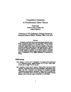
Fig. 1: Replicator dynamics of the pigeon orientation game The replicator dynamics enables us to display the evolutionary behavior of a game graphically. This has a considerable heuristic value. There are basically two techniques for this. First, it is possible to depict time series in a Cartesian coordinate system. The time is mapped to the x-axis, while the y-axis corresponds to the relative frequency of some strategy. For some sample of initial conditions, the development of the relative frequencies over time is plotted as a function of the time variable. In a two-strategy game like the pigeon orientation scenario discussed above, this is sufficient to exhaustively display the dynamics of the system because the relative frequencies of the two strategies always sum up to 1. Figure 1 gives a few sample time series for the pigeon game. Here the y-axis corresponds to the relative frequency of the A-population. It is plainly obvious that the state where 100% of the population are of type A is in fact an attractor. Another option to graphically display the replicator dynamics of some game is to suppress the time dimension and instead plot possible trajectories (also called orbits) of the system. Here both axes correspond to relative frequencies of some strategies. So each state of the population corresponds to some point in the coordinate system. If there are at most two independent variables to consider—as in a symmetric three-strategy game like RPS—there is actually a 1-1 map between points and states. Under the replicator dynamics, populations evolve continuously. This corresponds to contiguous paths in the graph. Figure 2 on the next page shows some trajectories of RPS. We plotted the frequencies of


10

R

S Fig. 2: Replicator dynamics of the rock-paper-scissor game the “rock” strategy and the “scissor” strategy against the y-axis and the x-axis respectively. The sum of their frequencies never exceeds 1. This is why the whole action happens in the lower left corner of the square. The relative frequency of “paper” is uniquely determined by the two other strategies and is thus no independent variable. The circular nature of this dynamics that we informally uncovered above is clearly to discern. One can also easily see “with the bare eye” that this game has no attractor, i.e., no ESS. There are plenty of different softwares on the market to produce such plots. We used the freely available program “Gnuplot” (combined with some numerical script language like “Octave” or “Python” to do the actual numerical computations) for the graphics shown here. There are also various commercial programs like “Mathematica” or “Matlab” which have more options (and are better documented!).

2.3

Asymmetric games

So far we considered symmetric games. Formally, a game is symmetric if the two players have the same set of strategies to choose from, and the utility does


11

H D

H D 1 7 2 3

Tab. 3: Hawks and Doves not depend on the position of the players. If u1 is the utility matrix for the row player, and u2 of the column player, then the game is symmetric iff both matrices are square (have the same number of rows and columns), and u1 (i, j) = u2 (j, i) There are various scenarios where these assumptions are inappropriate. In many types of interaction, the participants assume certain roles. In contests over a territory, it makes a difference who is the incumbent and who the intruder. In economic interaction, buyer and seller have different options at their disposal. Likewise in linguistic interaction you are the speaker or the hearer. The last example illustrates that it is possible for the same individual to assume either role at different occasions. If this is not possible, we are effectively dealing with two disjoint populations, like predators and prey or females and males in biology, haves and have-nots in economics, and adults and infants in language acquisition (in the latter case infants later become adults, but these stages can be considered different games). The dynamic behavior of asymmetric games differs markedly from symmetric ones. The ultimate reason for this is that in a symmetric game, an individual can quasi play against itself (or against a clone of himself), while this is impossible in asymmetric games. The well-studied game “Hawks and Doves” may serve to illustrate this point. Imagine a population where the members have frequent disputes over some essential resource (foot, territory, mates, whatever). There are two strategies to deal with a conflict. The aggressive type (the “hawks”) will never give in. If two hawks come in conflict, they fight it out until one of them dies. The other one gets the resource. The doves, on the contrary, embark upon a lengthy ritualized dispute until one of them is tired of it and gives in. If a hawk and a dove meet, the dove gives in right away and the hawk gets the resource without any effort. There are no other strategies. A possible utility matrix for this game is given in Table 3. Getting the disputed resource without effort has a survival value of 7. Only a hawk meeting a dove is as lucky. Not getting the resource at all without a fight enables the loser to look out for a replacement. This is the fate of a dove meeting a hawk. Lets say this has a utility of 2. Dying in a fight over the resource leads to an expected number of 0 offspring, and a serious fight is also costly for the survivor. Let us say the average utility of a hawk meeting a hawk is 1. A dove meeting another dove will get the contested resource in one out of two occasions


12

1

0.8

0.6

0.4

0.2

0

t

Fig. 3: Symmetric Hawk-and-Dove game on average, but the lengthy ritualistic contest comes with a modest cost too, so the utility of a dove meeting a dove could be 3. It is important to notice that the best response to a hawk is being a dove and vice versa. So neither of the two pure strategies is an NE. However, we also consider mixed strategies where either the population is mixed, or each individual plays either strategy with a certain probability. Under these circumstances, the game has an ESS. If the probability of behaving like a hawk is 80% and of being a dove 20%, both strategies achieve an expected utility of 2.2. As the reader may convince herself, this mixed strategy does in fact fulfill the conditions for an ESS. The replicator dynamics is given in Figure 3. Here the x-axis represents the proportion of hawks in a population. If the proportion of hawks exceeds the critical 80%, doves have an advantage and will spread, and vice versa. This changes dramatically if the same game is construed as an asymmetric game. Imagine the same situation as before, but now we are dealing with two closely related but different species. The two species are reproductively isolated, but they compete for the same ecological niche. Both species come in the hawkish and the dovish variant. Contests only take place between individuals from different species. Now suppose the first species, call it A, consists almost exclusively of the hawkish type. Under symmetric conditions, this would mean that the hawks mostly encounter another hawk, doves are better off on average, and therefore evolution works in favor of the doves. Things are different in the asymmetric situ-


13

Fig. 4: Asymmetric Hawk-and-Dove game ation. If A consists mainly of hawks, this supports the doves in the other species, B. So the proportion of doves in B will increase. This in turn reinforces the dominance of hawks in A. Likewise, a dominantly dovish A-population helps the hawks in B. The tendency works always in favor of a purely hawkish population in the one species and a purely dovish population in the other one. Figure 4 graphically displays this situation. Here we use a third technique for visualizing a dynamics, a direction field. Each point in the plain corresponds to one state of the system. Here the x-coordinate gives the proportion of hawks in A, and the y-coordinate the proportion of hawks in B. Each arrow indicates in which direction the system is moving if it is in the state corresponding to the origin of the arrow. The length of the arrow indicates the velocity of the change. If you always follow the direction of the arrows, you get a trajectory. Direction fields are especially useful to display systems with two independent variables, like the two-population game considered here. The system has two attractor states, the upper left and the lower right corner. They correspond to a purely hawkish population in one species and 100% doves in the other. If both populations have the critical 8:2 ratio of hawks:doves that was stable in the symmetric scenario, the system is also stationary. But this is not an attractor state because all points in the environment of this point are pulled away from it rather than being attracted to it. It is possible to capture the stability properties of asymmetric games in a way that is similar to the symmetric case. Actually the situation is even easier in


14

the asymmetric case. The definition of a symmetric ESS was complicated by the consideration that mutants may encounter other mutants. In a two-population game, this is impossible. In a one-population role game, this might happen. However, minimal mutations only affect strategies in one of the two roles. If somebody minimally changes his grammatical preferences as a speaker, say, his interpretive preferences need not be affected by this.5 So while a mutant might interact with its clone, it will never occur that a mutant strategy interacts with itself, because, by definition, the two strategy sets are distinct. So, the second clause of the definition of ESS doesn’t matter. We have to make some conceptual adjustments for the asymmetric case. Since the two strategy sets are distinct, the utility matrices are distinct as well. In a game between m and n strategies, the utility function of the first player is defined by an m × n matrix, call it uA , and an n × m matrix uB for the second player. An asymmetric Nash Equilibrium is now a pair of strategies, one for each population/role, such that each component is the best response to the other component. Likewise, a SNE is a pair of strategies where each one is the unique best response to the other. Now if the second clause in the definition of a symmetric ESS plays no role here, does this mean that only the first clause matters? In other words, are all and only the NEs evolutionarily stable in the asymmetric case? Not quite. Suppose a situation as before, but now species A consists of three variants instead of two. The first two are both aggressive, and they both get the same, hawkish utility. Also, individuals from B get the same utility from interacting with either of the two types of hawks in A. The third A-strategy are still the doves. Now suppose that A consists exclusively of hawks of the first type, and B only of doves. Then the system is in an NE, since both hawk strategies are the best response to the doves in B, and for a B-player, being a dove is the best response to either hawkstrategy. If this A-population is invaded by a mutant of the second hawkish type, the mutants are exactly as fit as the incumbents. They will neither spread nor be extinguished. (Biologists call this phenomenon drift—change that has no impact for survival fitness and is driven by pure chance.) In this scenario, the system is in a (non-strict) NE, but it is not evolutionarily stable. A strict NE is always evolutionarily stable though, and it can be shown (Selten 1980) that : In asymmetric games, a configuration is an ESS iff it is a SNE. It is a noteworthy fact about asymmetric games that ESSs are always pure in the sense that both populations play one particular strategy with 100% probability. This does not imply though that asymmetric games always settle in a 5

One might argue that the strategies of a language user in these two roles are not independent. If this correlation is deemed to be important, the whole scenario has to be formalized as a symmetric game. See below for techniques of how to symmetrize asymmetric games.


15

pure state. Not every asymmetric game has an ESS. The asymmetric version of rock-paper-scissor, for instance, shows the same kind of cyclic dynamics as the symmetric variant. As in the symmetric case, this characterization of evolutionary stability is completely general and holds for all utility monotonic dynamics. Again, the simplest instance of such a dynamic is the replicator dynamic. Here a state is characterized by two probability vectors, x and y. They represent the probabilities of the different strategies in the two populations or roles. By similar considerations as above, the dynamics of the asymmetric replicator dynamics can be described by the system of differential equations: n m n X X X dxi = xi ( yj uA (i, j) − xk yj uA (k, j)) dt j=1 j=1 k=1

(12)

m n m X X X dyi = yi ( xj uB (i, j) − yk xj uB (k, j)) dt j=1 j=1 k=1

(13)

It is straightforward to transform an asymmetric game into a symmetric game. In the previous setup, we had a population A with m strategies and a utility matrix ua , interacting with a population B with n strategies and a utility matrix uB . We may construct the set of pairs from A and B respectively and consider each such pair as a member of an abstract meta-population, being engaged in a meta-game. Every pair of interactions in the original game corresponds to one interaction in the meta-game. If a1 interacted with b1 and a2 with b2 in the original game, this amounts to an interaction of ha1 , b2 i with ha2 , b1 i in the new game. If SA and SB are the strategy sets in the original game, the meta-game has just one such set, SA ∪ SB . Since SA and SB are disjoint by definition, there are m + n meta-strategies. The utility of a combined strategy is the sum of the utilities of the component strategies. If we call the meta-utility function uAB , we have uAB (hi, ji, hk, li) = uA (i, l) + uB (j, k) The meta-game is a symmetric game. It turns out that the replicator dynamics of the meta-population can be described by the standard symmetric replicator dynamics. Also every SNE, this is, every ESS, in the original game corresponds to an ESS in the meta-game. So the essential dynamic characteristics of an asymmetric game are thus preserved when it is symmetrized. On the other hand, reducing a symmetric game to an asymmetric one is not possible. This is probably the reason why asymmetric games are usually not given much attention in the literature. For practical purposes, it does make quite a difference though whether you have to deal with a 3 × 10 asymmetric game, say, or with the 30 × 30 symmetrized version of it. Especially applications of GT in linguistic pragmatics frequently deal with the

3 EGT and language

16

asymmetry between speaker and hearer. A formalization as asymmetric game might thus be more natural here. Also, in more sophisticated dynamic models like spatial EGT, an asymmetric game need not be reducible to a symmetric one.

3

EGT and language

Natural language is an interactive and self-replicative system. This makes EGT a promising analytical tool for the study of linguistic phenomena. Let us start this section with a few general remarks. To give an EGT formalization—or an evolutionary conceptualization in general—of a particular empirical phenomenon, various issues have to be addressed in advance. What is replication in the domain in question? What are the replicators? Is replication faithful, and if so, which features are constant under replication? What factors influence reproductive success (= fitness)? What kind of variation exists, and how does it interact with replication? There are various aspects of natural language that are subject to replication, variation and selection, on various timescales that range from minutes (single discourse) till millennia (language related aspects of biological evolution). We will focus on cultural (as opposed to biological) evolution on short time scales, but we will briefly discuss the more general picture. The most obvious mode of linguistic self-replication is first language acquisition. Before this can take effect, the biological preconditions for language acquisition and use have to be given, ranging from the physiology of the ear and the vocal tract to the necessary cognitive abilities. The biological language faculty is replicated in biological reproduction. It seems obvious that the ability to communicate does increase survival chances and social standing and thus promotes biological fitness, but only at a first glance. Sharing information usually benefits the receiver more than the sender. Standard EGT predicts this kind of altruistic behavior to be evolutionarily unstable. Here is a crude formalization in terms of an asymmetric game between sender and receiver. The sender has a choice between sharing information (“T” for “talkative”) or keeping information for himself (“S” for “silent”). The (potential) receiver has the options of paying attention and trying to decode the messages of the sender (“A” for “attention”) or to ignore (“I”) the sender. Let us say that sharing information does have a certain benefit for the sender because it may serve to manipulate the receiver. On the other hand, sending a signal comes with an effort and may draw the attention of predators. For the sake of the argument, we assume that the costs and benefits are roughly equally distributed given the receiver pays attention. If the receiver ignores the message, it is disadvantageous for the sender to be talkative. For the receiver, it pays to pay attention if the sender actually sends. Then the listener benefits most. If the sender is silent, it is of disadvantage for the listener to pay attention because attention is a precious resource that could have been

3 EGT and language

17

T S

A I 1,2 0,1 1,0 1,1

Tab. 4: The utility of communication spend in a more useful way otherwise. Sample utilities that mirror these assumed preferences are given in Table 4. Here the two utility matrices are written in one table. The first number in each cell represents the utility of the row player (the sender) and the second one the utility of the column player (the receiver). The game has exactly one ESS, namely the combination of “S” and “I”. (As the careful reader probably already figured out for herself, a cell is an ESS, i.e., an strict Nash equilibrium, if its first number is the unique maximum in its column and the second one the unique maximum in its row.) This result might seem surprising. The receiver would actually be better off if the two parties would settle at (T,A). This would be of no disadvantage for the sender. Since the sender does not compete with the receiver for resources (we are talking about an asymmetric game), he could actually afford to be generous and grant the receiver the possible gain. Here the predictions of standard EGT seem to be at odds with the empirical observations.6 The evolutionary basis for communication, and for cooperation, is an active area of research in EGT, and there are various possible routes that have been proposed. First, the formalization that we gave here may be just wrong, and communication is in fact beneficial for both parties. While this is certainly true for humans living in human societies, this still raises the questions how these societies could have evolved in the first place. A more interesting approach goes under the name of the handicap principle. The name was coined by Zahavi (1975) to describe certain patterns of seemingly self-destructive communication in the animal kingdom. For instance, gazelles sometimes don’t run away immediately when they spot a lion but do certain mock dances that are visible for the lion. Only a gazelle that is fit enough to outrun the lion even if it does some dancing before can afford such a behavior. For a slow gazelle such a behavioral pattern could end lethally. The best reply for the lion would then be not to chase the gazelle because it would only mean a waste of time and energy. To be more precise, the best response of the lion is to call the bluff occasionally, often enough to deter cheaters, but not too often. Under these conditions, the self-inflicted handicap of the (fast) gazelle is in fact evolutionarily stable. So the evolutionarily stable strategies for fast gazelles would be to dance in face of the lion, while the best thing to do for a slow gazelle is to run as soon and 6

This problem is related to the well-worn prisoners dilemma, where standard EGT also predicts the egotistic strategy to be the only evolutionarily stable one.

3 EGT and language

18

as fast as possible. Given this, the dance is a form of communication between the gazelle and the lion, expressing “I am faster than you”. The crucial insight here is that truthful communication can be evolutionarily stable if lying is more costly than communicating the truth. A slow gazelle could try to use the mock dance as well to discourage a lion from hunting it, but this would be risky if the lion occasionally calls the bluff. The expected costs of such a strategy are thus higher than the costs of running away immediately. In communication among humans, there are various way how lying might be more costly than telling (or communicating) the truth. To take an example from economics, driving a Rolls Royce communicates “I am rich” because for a poor man, the costs of buying and maintaining such an expensive car outweigh its benefits while a rich man can afford them. Here producing the signal as such is costly. In linguistic communication, lying comes with the social risk of being found out, so in many cases telling the truth is more beneficial than lying. The idea of the handicap principle as evolutionary basis for communication has inspired a plethora of research in biology and economics. Van Rooij (2003) uses it to give a game theoretic explanation of politeness as a pragmatic phenomenon. A third hypothesis rejects the assumption of standard EGT that all individuals interact with equal probability. When I increase the fitness of my kin, I thereby increase the chances for replication of my own gene pool, even if it should be to my own disadvantage. Recall that utility in EGT does not mean the reproductive success of an individual but of a strategy, and strategies correspond to heritable traits in biology. A heritable trait for altruism might thus have a high expected utility provided its carriers preferably interacts with other carriers of this trait. Biologists call this model kin selection. There are various modifications of EGT that give up the assumption of random pairing. We will return to this issue later on. Natural languages are not passed on via biological but via cultural transmission. First language acquisition is thus a qualitatively different mode of replication. Most applications of evolutionary thinking in linguistics focus on the ensuing acquisition driven dynamics. It is an important aspect in understanding language change on a historical timescale of decades and centuries. It is important to notice that there is a qualitative difference between Darwinian evolution and the dynamics that results from iterated learning (in the sense of iterated first language acquisition). In Darwinian evolution, replication is almost always faithful. Variation is the result of occasional unfaithful replication, a rare and essentially random event. Theories that attempt to understand language change via iterated language acquisition stress the fact though that here, replication can be unfaithful in a systematic way. The work of Martin Nowak and his co-workers (see for instance Nowak et al. 2002) is a good representative of this approach. They assume that an infant that grows up in a community of speaker of some language L1 might acquire another language L2 with a certain

3 EGT and language

19

probability. This means that those languages will spread in a population that (a) are likely targets of acquisition for children that are exposed to other languages, and (b) are likely to be acquired faithfully themselves. This approach thus conceptualizes language change as a Markov process7 rather than evolution through natural selection. Markov processes and natural selection of course do not exclude each other. Nowak’s differential equation describing the language acquisition dynamics actually consist of a basically game theoretical natural selection component (pertaining to the functionality of language) and a (learning oriented) Markov component. Language gets replicated on a much shorter time scale, just via being used. The difference between acquisition based and usage based replication can be illustrated by looking at the development of the vocabulary of some language. There are various ways how a new word can enter a language—morphological compounding, borrowing from other languages, lexicalization of names, coinage of acronyms, what have you. Once a word is part of a language, it is gradually adapted to this language, i.e., it acquires a regular morphological paradigm, its pronunciation is nativized etc. The process of establishing a new word is predominantly driven by mature (adult or adolescent) language users, not by infants. Somebody introduces the new word, and people start imitating it. Whether the new coinage catches on depends on whether there is a need for this word, whether it fills a social function (like distinguishing the own social group from other groups), on the social prestige of the persons who already use it etc. Since the work of Labov (see for instance Labov 1972) functionally oriented linguists have repeatedly pointed out that grammatical change actually follows a similar pattern. The main agents of language change, they argue, are mature language users rather than children.8 Not just the vocabulary is plastic and changes via language use but all kinds of linguistic variables like syntactic constructions, phones, morphological devices, interpretational preferences etc. Imitation plays a crucial part here, and imitation is of course a kind of replication. Unlike in biological replication, the usage of a certain word or construction can usually not be traced back to a unique model or pair of models that spawn the token in question. Rather, every previous usage of this linguistic item that the user took notice of shares a certain fraction of “parenthood”. Recall though that the basic units of evolution in EGT are not individuals but strategies, and evolution is about the relative frequency of strategies. If there is a causal relation between the abundance of a certain linguistic variant at a given point in time and its abun7 A Markov process is a stochastic process where the system is always in one of finitely many states, and where the probability of the possible future behaviours of the system only depends on its current state, not on its history. 8 If true, this of course entails that the linguistic competence of adult speaker remains plastic. While this seems to be at odds with some versions of generative grammar, the work of Tony Kroch (see for instance Kroch 2000) shows that this is perfectly compatible with a principles-and-parameters conception of grammar.

4 Pragmatics and EGT

20

dance at a later point, we can consider this a kind of faithful replication. Also, replication is almost but not absolutely faithful. This leads to a certain degree of variation. Competing variants of a linguistic item differ in their likelihood to be imitated—this corresponds to fitness and thus to natural selection. The usage based dynamics of language use has all aspects that are required for a modeling in terms of EGT. In the linguistic examples that we will discuss further on, we will assume the latter notion of linguistic evolution.

4

Pragmatics and EGT

In this section we will go through a couple of examples that demonstrate how EGT can be used to explain high level linguistic notions like pragmatic preferences or functional pressure.

4.1

Partial blocking

If there are two comparable expressions in a language such that the first is strictly more specific than the second, there is a tendency to reserve the more general expression for situations where the more specific one is not applicable. A standard example is the opposition between “many” and “all”. If I say that many students came to the guest lecture, it is usually understood that not all students came. There is a straightforward rationalistic explanation for this in terms of conversational maxims: the speaker should be as specific as possible. If the speaker uses “many”, the hearer can conclude that the usage of “all” would have been inappropriate. This conclusion is strictly speaking not valid though—it is also possible that the speaker just does not know whether all students came or whether a few were missing. A similar pattern can be found in conventionalized form in the organization of the lexicon. If a regular morphological derivation and a simplex word compete, the complex word is usually reserved for cases where the simplex is not applicable. For instance, the compositional meaning of the English noun “cutter” is just someone or something that cuts. A knife is an instrument for cutting, but still you cannot call a knife a “cutter”. The latter word is reserved for non-prototypical cutting instruments. Let us consider the latter example more closely. We assume that the literal meaning of “cutter” is a concept cutter’ and the literal meaning of “knife” a concept knife’ such that every knife is a cutter but not vice versa, i.e., knife’ ⊂ cutter’ There are two basic strategies to use these two words, the semantic (S) and the pragmatic (P ) strategy. Both come in two versions, a hearer strategy and


21

a speaker strategy. A speaker using S will use “cutter” to refer to unspecified cutting instruments, and “knife” to refer to knifes. To refer to a cutting instrument that is not a knife, this strategy either uses the explicit “cutter but not a knife”, or, short but imprecise, also “cutter”. A hearer using S will interpret every expression literally, i.e., “knife” means knife’, “cutter” means cutter’, and “cutter but not a knife” means cutter’ − knife’. A speaker using P will reserve the word “cutter” for the concept cutter’ − knife’. To express the general concept cutter’, this strategy has to take resort to a more complex expression like “cutter or knife”. Conversely, a hearer using P will interpret “cutter” as cutter’ − knife’, “knife” as knife’, and “cutter or knife” as cutter’. So we are dealing with an asymmetric 2 × 2 game. What is the utility function? In EGT, utilities are interpreted as the expected number of offspring. In our linguistic interpretation this means that utilities express the likelihood of a strategy to be imitated. It is a difficult question to tease apart the factors that determine the utility of a linguistic item in this sense, and ultimately it has to be answered by psycholinguistic and sociolinguistic research. Since we have not undertaken this research so far, we will make up a utility function, using plausibility arguments. We start with the hearer perspective. The main objective of the hearer in communication, let us assume, is to gain as much truthful information as possible. The utility of a proposition for the hearer is thus inversely proportional to its probability, provided the proposition is true. For the sake of simplicity, we only consider contexts where the nouns in question occur in upward entailing context. Therefore cutter’ has a lower information value than knife’ or cutter’−knife’. It seems also fair to assume that non-prototypical cutters are rarer talked about than knifes; thus the information value of knife’ is lower than the one of cutter’−knife’. For concreteness, we make up some numbers. If i is the function that assigns a concept its information value, let us say that i(knife’) = 30 i(cutter’ − knife’) = 40 i(cutter’) = 20

The speaker wants to communicate information. Assuming only honest intentions, the information value that the hearer gains should also be part of the speaker’s utility function. Furthermore, the speaker wants to minimize his effort though. So as a second component of the speaker’s utility function, we assume some complexity measure over expressions. A morphologically complex word like “cutter” is arguably more complex than a simple one like “knife”, and syntactically complex phrases like “cutter or knife” or “cutter but not knife” are even


22

S P

S P 23.86, 28.60 24.26, 29.00 23.40, 29.00 25.40, 31.00 Tab. 5: knife vs. cutter

more complex. The following stipulated values for the cost function take these considerations into account: cost(“knife”) cost(“cutter”) cost(“cutter or knife”) cost(“cutter but not knife”)

= = = =

1 2 40 45

These costs and benefits are to be weighted—everything depends on how often each of the candidate concepts is actually used. The most prototypical concept of the three is certainly knife’, while the unspecific cutter’ is arguably rare. Let us say that, conditioned to all utterance situations in question, the probabilities that a speaker tries to communicate the respective concepts are p(knife’) = .7 p(cutter’ − knife’) = .2 p(cutter’) = .1

The utility of the speaker is then the difference between the average information value that he manages to communicate and the average costs that he has to afford. The utility of the hearer is just the average value of the correct information that is received. The precise values of these utilities finally depend on how often a speaker of the S-strategy actually uses the complex “cutter but not knife”, and how often he uses the shorter “cutter”. Let us assume for the sake of concreteness that he uses the short form in 60% of all times. After some elementary calculations, this leads us to the following utility matrix. The speaker is assumed to be the row player and the hearer the column player. As always, the first entry in each cell gives the utility of the row player, i.e., the speaker. Both players receive the absolutely highest utility if both play P . This means perfect communication with minimal effort. All other combinations involve some kind of communication failure because the hearer either interprets the speaker’s use of “cutter” either too strong or too weak occasionally.


23

Fig. 5: Partial blocking: replicator dynamics If both players start out with the semantic strategy, mutant hearers that use the pragmatic strategy will spread because they get the more specific interpretation cutter’−knife’ right in all cases where the speaker prefers minimizing effort over being explicit. The mutants will get all cases wrong where the speaker meant cutter’ by using “cutter”, but the advantage is greater. If the hearers employ the pragmatic strategy, speakers using their pragmatic strategy will start to spread now because they will have a higher chance to get their message across. The combination P/P is the only strict Nash equilibrium in the game and thus the only ESS. Figure 5 gives the direction field of the corresponding replicator dynamics. The x-axis gives the proportion of the hearers that are P -players, and the y-axis gives corresponds to the speaker dimension. The structural properties of this game are very sensitive to the particular parameter values. For instance, if the informational value of the concept cutter’ were 25 instead of 20, the resulting utility matrix would come out as in Table 6 on the next page. Here both S/S and P/P come out as evolutionarily stable. This result is not entirely unwelcome—there are plenty of examples where a specific term does not block a general term. If I refer to a certain dog as “this dog”, I do not implicate that it has no discernible race like “German shepherd” or “Airedale


24

S P

S P 24.96, 29.70 24.26, 29.00 23.40, 30.00 25.90, 31.50

Tab. 6: knife vs. cutter, different parameter values terrier”. The more general concept of a dog is useful enough to prevent blocking by more specific terms.

4.2

Horn strategies9

Real synonymy is rare in natural language—some people even doubt that it exists. Even if two expression should have identical meanings according to the rules of compositional meaning interpretations, their actual interpretation is usually subtly differentiated. Larry Horn (see for instance Horn 1993) calls this phenomenon the division of pragmatic labor. This differentiation is not just random. Rather, the tendency is that the simpler of the two competing expressions is assigned to the prototypical instances of the common meaning, while the more complex expression is reserved for less prototypical situations. The following examples (taken from op. cit.) serve to illustrate this. (1)

a. b.

John went to church/jail. (prototypical interpretation) John went to the church/jail. (literal interpretation)

(2)

a. b.

I will marry you. (indirect speech act) I am going to marry you. (no indirect speech act)

(3)

a. b.

I need a new driller/cooker. I need a new drill/cook.

The example (1a) only has the non-literal meaning where John attended a religious service or was convicted to a prison sentence respectively. The more complex (b) sentence literally means that he approach the church (jail) as a pedestrian. In (2), the simpler (a) version represents an indirect speech act of a promise, but the more complex (b) is just an ordinary assertion. De-verbal nouns formed by the suffix -er can either be agentive or refer to instruments. So compositionally, a driller could be a person who drills or an instrument for drilling, and likewise for cooker. However, drill is lexicalized as a drilling instrument, and thus driller can only have the agentive meaning. For cooker it is the other way round: a cook is a person who cooks, and thus a cooker 9

The material in this subsection draws heavily on van Rooij (2004)


25

can only be an instrument. Arguably the concept of a person who cooks is a more natural concept than an instrument for cooking in our culture, and for drills and drillers it is the other way round. So in either case, the simpler form is restricted to the more prototypical meaning. One might ask what “prototypical” exactly means here. The meaning of “going to church” for instance is actually more complex than the meaning of “going to the church” because the former invokes a lot of cultural background knowledge. It seems to make sense to us though to simply identify prototypicality with frequency. Those meanings that are most often communicated in ordinary conversations are most prototypical. We are not aware whether anybody ever did quantitative studies on this subject, but simple Google searches show that for the mentioned examples, this seems to be a good hypothesis. The phrase “went to church” got 88,000 hits, against 13,500 for “went to the church”. “I will marry you” occurs 5,980 times; “I am going to marry you” only 442 times. “A cook” has about 712,000 occurrences while “a cooker” has only about 25,000. (This crude method is not applicable to “drill” vs. “driller” because the former also has an additional meaning as in “military drill” which pops up very often.) While queries at a search engine do not replace serious quantitative investigations, we take it to be a promising hypothesis that in case of a pragmatic competition, the less complex form tends to be restricted to the more frequent meaning and the more complex one to the less frequent interpretation. It is straightforward to formalize this setting in a game. The players are speaker and hearer. There are two meanings that can be communicated, m0 and m1 , and they have two forms at their disposal, f0 and f1 . Each total function from meanings to forms is a speaker strategy, while hearer strategies are mappings from forms to meanings. There are four strategies for each player, as shown in Table 7 on the following page. It is decided by nature which meaning the speaker has to communicate. The probability that nature chooses m0 is higher than the probability of m1 . Furthermore, form f0 is less complex than form f1 . The players both have the goal to successfully communicate the meaning that nature provides from the speaker to the hearer. Furthermore, the speaker has an interest in minimizing the complexity of the expression involved. One might argue that the hearer also has an interest in minimizing complexity. However, the hearer is confronted with a given form and has to make sense of it. He or she has no way to influence the complexity of that form or the associated meaning. Therefore there is no real point in making complexity part of the hearer’s utility function. To keep things simple, let us make up some concrete numbers. Let us say that the probability of m1 is 75% and the probability of m2 25%. The costs of f1 and f2 are 0.1 and 0.2 respectively. The unit is the reward for successful communication—so we assume that it is 10 times as important for the speaker to get the message across than to avoid the difference in costs between f2 and


26

Speaker

Hearer

S1:

m0 → 7 f0 m1 → 7 f1

H1:

f0 → 7 m0 f1 → 7 m1

S2:

m0 → 7 f1 m1 → 7 f0

H2:

f0 7→ m1 f1 7→ m0

S3:

m0 → 7 f0 m1 → 7 f0

H3:

f0 7→ m0 f1 7→ m0

S4:

m0 → 7 f1 m1 → 7 f1

H4:

f0 7→ m1 f1 7→ m1

Tab. 7: Strategies in the Horn game f1 . We exclude strategies where the speaker does not say anything at all, so the minimum costs of 0.1 unit is unavoidable. The utility of the hearer for a given pair of a hearer strategy and a speaker strategy is the average number of times that the meaning comes across correctly given the strategies and nature’s probability distribution. Formally this means that uh (H, S) =

X

pm × δm (S, H)

m

where the δ-function is defined as (

δm (S, H) =

1 iff H(S(m)) = m 0 else

The speaker shares the interest in communicating successfully, but he also wants to avoid costs. So his utility function comes out as us (S, H) =

X m

pm × (δm (S, H) − cost(S(m)))


S1 S2 S3 S4

H1 .875 -.175 .65 .05

27

1.0 0.0 .75 .25

H2 -.125 .825 .15 .55

0.0 1.0 .25 .75

H3 H4 .625 .75 .125 .25 .575 .75 .25 .075 .65 .75 15 .25 .55 .75 .05 .25

Tab. 8: Utility matrix of the Horn game With the chosen numbers, this gives us the utility matrix in Table 8. The first question that might come to mind is what negative utilities are supposed to mean in EGT. Utilities are the expected number of offspring—what is negative offspring? Recall though that if applied to cultural language evolution, the replicating individuals are utterances, and the mode of replication is imitation. Here the utilities represent the difference in the absolute abundance of a certain strategy at a given point in time and at a later point. A negative utility thus simply means that the number of utterances generated by a certain strategy is absolutely declining. Also, neither the replicator dynamics nor the locations of ESSs or Nash equilibria change if a constant amount is added to all utilities within a matrix. It is thus always possible to transform any given matrix into an equivalent one with only non-negative entries. We are dealing with an asymmetric game. Here all and only the strict Nash equilibria are evolutionarily stable. There are two such stable states in the game at hand: (S1 , H1 ) and (S2 , H2 ). As the reader may verify, these are the two strategy configurations where both players use a 1-1 function, the hearer function is the inverse of the speaker function, and where thus communication always succeeds. EGT thus predicts the emergence of a division of pragmatic labor. It does not predict though that the “Horn strategy” (S1 , H1 ) is in any way superior to the “anti-Horn strategy” (S2 , H2 ) where the complex form is used for the frequent meaning. There are various reasons why the former strategy is somehow “dominant”. First, it is Pareto-efficient. This means that for both players, the utility that they get if both play Horn is at least as high as in the other ESS where they both play anti-Horn. For the speaker Horn is absolutely preferable. Horn also risk-dominates anti-Horn. This means that if both players play Horn, either one would have to lose a lot by deviating unilaterally to antiHorn, and this “risk” is at least as high as the inverse risk, i.e., the loss in utility from unilaterally deviating from the anti-Horn equilibrium. For the speaker, this dominance is strict. However, these considerations are based on a rationalistic conception of GT, and they are not directly applicable to EGT. There are two arguments for the dominance of the Horn strategy that follow directly from the replicator dynamics. • A population where all eight strategies are equally likely will converge

5 All equilibria are stable, but some equilibria are more stable than others: Stochastic EGT 28

towards a Horn strategy. Figure 6 on the following page gives the time series for all eight strategies if they all start at 25% probability. Note that the hearers first pass a stage where strategy H3 is dominant. This is the strategy where the hearer always “guesses” the more frequent meaning— a good strategy as long as the speaker is unpredictable. Only after the speaker starts to clearly differentiate between the two meanings does H1 begin to flourish. • While both Horn and anti-Horn are attractors under the replicator dynamics, the former has a much larger basin of attraction than the latter. We are not aware of a simple way of analytically calculating the ratio of the sizes of the two basins, but a numerical approximation revealed that the basin of attraction of the Horn strategy is about 20 times as large as the basin of attraction of the anti-Horn strategy. The asymmetry between the two ESSs becomes even more apparent when the idealizations “infinite population” and “complete random mating” are lifted. In the next sections we will briefly explore the consequences of this.

5

All equilibria are stable, but some equilibria are more stable than others: Stochastic EGT

Let us now have a closer look at the modeling of mutations in EGT. Evolutionary stability means that a state is stationary and resistant against small amounts of mutations. This means that the replicator dynamics is tacitly assumed to be combined with a small stream of mutation from each strategy to each other strategy. The level of mutation is assumed to be constant. An evolutionarily stable state is a state that is an attractor in the combined dynamics and remains an attractor as the level of mutation converges towards zero. The assumption that the level of mutation is constant and deterministic though is actually an artifact of the assumption that populations are infinite and time is continuous in standard EGT. Real populations are finite, and both games and mutations are discrete events in time. So a more fine-grained modeling should assume finite populations and discrete time. Now suppose that for each individual in a population, the probability to mutate towards the strategy s within one time unit is p, where p may be very small but still positive. If the population consists of n individuals, the chance that all individuals end up playing s at a given point in time is at least pn , which may be extremely small but is still positive. By the same kind of reasoning, it follows that there is a positive probability for a finite population to jump from each state to each other state due to mutation (provided each strategy can be the target of mutation of each other strategy). More generally, in a finite population the stream of mutations is not constant but noisy and non-deterministic. Hence there are strictly speaking


1 0.9 0.8 0.7 0.6 0.5 0.4 0.3 0.2 0.1 0 -0.1 S1

S2

S3

S4

H1

H2

H3

H4

1 0.9 0.8 0.7 0.6 0.5 0.4 0.3 0.2 0.1 0 -0.1

Fig. 6: Time series of the Horn game


no evolutionarily stable strategies because every invasion barrier will eventually be overcome, no matter how low the average mutation probability and how high the barrier is.10 If an asymmetric game has exactly two SNEs, A and B, in a finite population with mutations there is a positive probability pAB that the system moves from A to B due to noisy mutation, and a probability pBA for the reverse direction. If pAB > pBA , the former change will on average occur more often than the latter, and in the long run the population will spend more time in state B than in state A. Put differently, if such a system is observed at some arbitrary time, the probability that it is in state B is higher than that it is in A. The exact value of this probability converges towards pABpAB as time grows to infinity. +pBA If the level of mutation gets smaller, both pAB and pBA get smaller, but at different pace. pBA approaches 0 much faster than pAB , and thus pABpAB +pBA (and thus the probability of the system being in state B) converges to 1 as the mutation rate converges to 0. So while there is always a positive probability that the system is in state A, this probability can become arbitrarily small. A state is called stochastically stable if its probability converges to a value > 0 as the mutation rate approaches 0. In the described scenario, B would be the only stochastically stable state, while both A and B are evolutionarily stable. The notion of stochastic stability is a strengthening of the concept of evolutionary stability; every stochastically stable state is also evolutionarily stable,11 but not the other way round. We can apply these considerations to the equilibrium selection problem in the Horn game from the last section. Figure 7 on page 32 shows the results of a simulation, using a stochastic dynamics in the described way.12 The figure on top shows the proportion of the Horn strategy S1 and the bottom figure the anti10

This idea has first been developed in Kandori et al. (1993) and Young (1993). Fairly accessible introductions to the theory of stochastic evolution are given in Vega-Redondo (1996) and Young (1998). 11 Provided the population is sufficiently large, that is. Very small populations may display a weird dynamic behavior, but we skip over this side aspect here. 12 The system of difference equations used in the experiment is ∆xi ∆t

= xi ((Ay)i − hx × Ayi) +

∆yi ∆t

= yi ((Bx)i − hy × Bxi) +

X Zji − Zij j

n

X Zji − Zij j

n

where x, y are the vectors of the relative frequencies of the speaker strategies and hearer strategies, and A and B are the payoff matrices of speakers and hearers respectively. For each pair of strategies i and j belonging to the same player, Zij gives the number of individuals that mutate from i to j. Zij is a random variable which is distributed according to the binomial distribution b(pij , bxi nc) (or b(pij , byi nc) respectively), where pij is the probability that an arbitrary individual of type i mutates to type j within one time unit, and n is the size of the population. We assumed that both populations have the same size.


Horn strategy S2 . The other two speaker strategies remain close to zero. The development for the hearer strategies is pretty much synchronized. During the simulation, the system spent 67% of the time in a state with a predominant Horn strategy and only 26% with predominant anti-Horn (the remaining time are the transitions). This seems to indicate strongly that the Horn strategy is in fact the more probable one, which in turn indicates that it is the only stochastically stable state. The literature contains some general results about how to find the stochastically stable states of a system analytically, but they are all confined to 2×2 games. This renders them practically useless for linguistic applications because here, even in very abstract models like the Horn game, we deal with more than two strategies per player. For larger games, analytical solutions can only be found by studying the properties in question on a case by case basis. It would take us too far to discuss possible solution concepts here in detail (see for instance Young 1998 or Ellison 2000). We will just sketch such an analytical approach for the Horn game, which turns out to be comparatively well-behaved. To check which of the two ESSs of the Horn game are stochastically stable, we have to compare the height of their invasion barriers. How many speakers must deviate from the Horn strategy such that even the smallest hearer mutation causes the system to leave the basin of attraction of this strategy and to move towards the anti-Horn strategy? And how many hearer-mutations would have this effect? The same questions have to be answered for the anti-Horn strategy, and the results to be compared. Consider speaker deviations from the Horn strategy. It will only lead to an incentive for the hearer to deviate as well if H1 is not the optimal response to the speaker strategy anymore. This will happen if at least 50% of all speakers deviate toward S2 , 66.7% deviate towards S4 , or some combination of such deviations. It is easy to see that the minimal amount of deviation having the effect in question is 50% deviating towards S2 .13 As for hearer deviation, it would take more than 52.5% mutants towards H2 to create an incentive for the speaker to deviate towards S2 , and even about 54% of deviation towards H4 to have the same effect. So the invasion barrier along the hearer dimension is 52.5%. Now suppose the system is in the anti-Horn equilibrium. As far as hearer utilities are concerned, Horn and anti-Horn are completely symmetrical, and thus the invasion barrier for speaker mutants is again 50%. However, if more than 47.5% of all hearers deviate towards H1 , the speaker has an incentive to deviate towards S1 . 13

Generally, if (si , hj ) form a SNE, the hearer has an incentive to deviate P from it as soon as the speaker chooses a mixed strategy x such that for some k = 6 j, i0 xi0 uh (si0 , hk ) > P 0 0 i0 xi uh (si , hj ). The minimal amount of mutants needed to drive the hearer out of the equilibrium would be the minmal value of 1 − xi for any mixed strategy x with this property. (The same applies ceteris paribus to mutations on the hearer side.)


1 0.9 0.8 0.7 0.6 0.5 0.4 0.3 0.2 0.1 0 Horn 1 0.9 0.8 0.7 0.6 0.5 0.4 0.3 0.2 0.1 0 anti-Horn

Fig. 7: Simulation of the stochastic dynamics of the Horn game

6 Don’t talk to strangers: Spatial EGT

33

In sum, the invasion barriers of the Horn and of the anti-Horn strategy are 50% and 47.5% respectively. Therefore a “catastropic” mutation from the latter to the former, though unlikely, is more likely than the reverse transition. This makes the Horn strategy the only stochastically stable state. In this particular example, only two strategies for each player played a role in determining the stochastically stable state. The Horn game thus behaves effectively as a 2 × 2 game. In such games stochastic stability actually coincides with the rationalistic notion of “risk dominance” that was briefly discussed above. In the general case, it is possible though that a larger game has two ESSs, but there is a possible mutation from one equilibrium towards a third state (for instance a non-strict Nash equilibrium) that lies within the basin of attraction of the other ESS. The stochastic analysis of larger games has to be done on a case-by-case basis to take such complex structures into account. In standard EGT, as well as in the version of Stochastic EGT discussed here, the utility of an individual at each point in time is assumed to be exactly the average utility this individual would get if it played against a perfectly representative sample of the population. Vega-Redondo (1996) discusses another variant of Stochastic EGT where this idealization is also given up. In this model, each individual plays a finite number of tournaments in each time step, and the gained utility—and thus the abundance of offspring—becomes a stochastic notion as well. He shows that this model sometimes leads to a different notion of stochastic stability than the one discussed here. A detailed discussion of this model would lead beyond the scope of this introduction though.

6

Don’t talk to strangers: Spatial EGT

Standard EGT assumes that populations are infinite and each pair of individuals is equally likely to interact. Stochastic gives up the first assumption. The second assumption is also quite unrealistic. Nowak and May (1992) give it up as well. Instead they assume that players are organized in a spatial structure. A simple model for this is a two-dimensional lattice like a chess board. Each player occupies one position in such a grid and interacts solely with its eight immediate neighbors. The overall utility of each player in each round is the sum of the utilities that it obtains in each of these eight interactions. In the next generation, each position in the grid adopts the strategy of the player in the immediate environment (the eight neighboring positions and the position in question itself) that obtained the highest utility. This kind of deterministic dynamics has a good deal of intrinsic mathematical interest because it leads to fascinating self-organizing behavior. Besides, various studies with different games and parameters invariably revealed that cooperative behavior performs much better in a spatial setting than in the standard model or in Stochastic EGT. There is a simple intuitive reason for this. Every individual


34

interacts with its spatial neighbors. The offspring of an individual are also always located in its immediate spatial proximity. Therefore individuals are likely to find their siblings or cousins in their environment. In a less metaphorical way of speaking, in the spatial setting strategies tend to cluster, and each individual is more likely to interact with somebody playing the same strategy than the population average would predict. Therefore those strategies that receive a high payoff against themselves have an advantage. Nowak and May’s pioneering paper, as well as most of the work that followed it (see for instance Killingback and Doebeli 1996), use the deterministic dynamics whereas each individual imitates the strategy with the highest utility in its spatial environment. We will use a perhaps more realistic non-deterministic version of spatial dynamics in the remainder of this section. The qualitative results of the mentioned studies remain valid in this setting. Recall that the utility is a measure for the expected number of offspring. If the offspring of an individual is distributed evenly over its spatial proximity, each cell in the lattice should adopt a mixed strategy—the combination of the strategies in its neighborhood in the previous generation, weighted according to their utility. We choose a slightly simpler model where each position is occupied by a pure strategy. The probability of adopting the strategy of a particular neighbor (or to retain the current strategy) is proportional to the utility of that neighbor. This approach is perhaps too simplistic though. Suppose strategy A obtains a utility of 10 against itself, while B only gets 5 points against itself. Then a homogeneous A-region should grow faster (because of its higher fitness) than a homogeneous B-region. This is not covered in the model so far. To remedy this, let us assume that each position can be populated by several individuals simultaneously. They are clones, i.e., they play the same strategy. The denser a position is populated, the higher is its impact on neighboring fields. To make this formally precise, let us assume a set of positions pos and a symmetric and irreflexive neighborhood relation n among elements of pos. The strategy function st maps positions and time points to a random variable over the strategy space. Likewise, the density function d maps positions and time points to a random variable over positive real numbers. Finally, the fitness function f maps positions and time points to positive reals as well. Z(a, t) is a normalization variable which holds the accumulated weighted fitness of the neighborhood of a. These random variables form a Markov process according to the following update rules:

f (a, t + 1) =

X

u(st(a, t), st(b, t))

b∈{x:n(a,x)}

d(a, t + 1) = d(a, t) × f (a, t + 1) 1 × P (st(a, t + 1) = i) = Z(a, t + 1)


35

C D

C D 5 1 8 2

Tab. 9: Utility matrix for the Prisoner’s Dilemma X

d(b, t + 1) × f (b, t + 1)

(b∈{x:n(a,x)}∪{a})∩{x:st(x,t)=i}

Z(a, t + 1) =

X

d(b, t + 1) × f (b, t + 1)

b∈{x:n(a,x)}∪{a}

It is a nice feature of this version of spatial dynamics that it is a refinement of the standard model. If the neighborhood of each point is identified with the entire set of positions, this dynamics converges towards the replicator dynamics as the number of positions grows to infinity. In the sequel we follow Nowak and May (1992) in assuming the two-dimensional lattice structure. Positions are arranged in a 50 × 50 grid. It is interpreted toroidal. This means that the top row neighbors the bottom row, and likewise for the leftmost and the rightmost column. Let us first consider the Hawk-andDove game discussed above. Recall that the only ESS in the standard model was 80% hawks vs. 20% doves. In the spatial setting, the dove strategy fares much better. Both strategies tend to form clusters. At the boundary between hawk populations and dove populations, hawks have the same advantage as in the classical setting. However, areas of dove sub-populations reach a higher density within a cluster than hawk areas because doves against doves have a utility of 3 while hawks against hawks only have a utility of 1. These two tendencies interact. Depending on the size of the clusters (which varies from generation to generation), the proportion of hawks in the entire population may reach its “classical” share of 80%, but it occasionally drops down to 50% and below. Figure 8 on the following page shows the relative proportion of hawks in a typical run of a simulation, starting from a state where both strategies are distributed randomly with equal probability over the range of positions. Here the divergence from the classical model was only gradual. In case of the prisoner’s dilemma, the spatial model(s) make(s) qualitatively different predictions. Recall that in the prisoner’s dilemma, we have two competing strategies, C (“Cooperate”) and D (“Defect”). C playing against C obtains a higher utility than D playing against D, but for a given strategy of the opponent, D always yields a higher payoff than C, no matter which strategy the opponent chooses. In technical vocabulary, D strictly dominates C, and therefore D is the only Nash equilibrium. Since it is a strict Nash equilibrium, it is also an ESS. Table 9 gives some concrete values that instantiate these preferences. Here the advantage that C-players enjoy if playing against other C-players


36

1

0.8

0.6

0.4

0.2

0

Fig. 8: Proportion of hawks in a spatial Hawk-and-Dove game

(T, A) (T, I) (S, A) (S, I)

(T, A) (T, I) (S, A) (S, I) 3 2 1 0 2 1 2 1 3 3 1 1 2 2 2 2

Tab. 10: Symmetrized game of communication is so overwhelming that it outweighs the disadvantage that ensues in direct encounters with defectors. Figure 9 on the following page shows the proportion of C-players in a simulation using the above utilities. We again started with an initial state where the strategies were assigned to positions at random with equal likelihood. In this state, there is little clustering, and most individuals interact with players using the other strategy. In this situation, D fares far better than C, and it almost takes over the entire space. However, some pockets of C-players survive and form clusters. Due to the high density inside these clusters, they constantly increase their size, until they finally occupy almost the entire space. The selection for cooperative behavior in spatial evolution is of obvious relevance for the evolution of communication. We briefly touched upon this issue in connection with the “game of communication” (see Table 4 on page 17). If we symmetrize this game, we get the utility matrix in Table 10. The only ESS here is (S, I), which corresponds to the only strict Nash equilibrium in the asymmetric version. The combination (T, I) is more beneficial for the hearer though and not worse than the ESS for the speaker. We thus have a


37

1

0.8

0.6

0.4

0.2

0

Fig. 9: Proportion of cooperators in a spatial Prisoner’s Dilemma game pattern that is similar to the prisoner’s dilemma. The ensuing spatial evolution is also similar. Starting from a random state, the ESS (S, I) quickly gains dominance and drives the other strategies close to extinction. In most simulations, some small clusters of the cooperative strategy (T, A) survive though. These clusters thrive and increase their size until they reach a stable shape. Under the grid structure used here, stable structures are squares or rectangles which are almost squares. The snapshots in figure 10 on the following page display the state of the system in the first, 11th, 25th, 100th, 200th and 500th generation. The strategy (S, I) is indicated by white squares and all other strategies by black squares. (T, I) and (S, A) die out after less than 30 generations; after that black squares just indicate (T, A). Interestingly, the equivalence between an asymmetric game and its symmetrized version breaks down under spatial evolution. In an asymmetric spatial competition, where players from both populations share one position in the lattice and each individual interacts with the individuals from the other population in its neighborhood, the classical ESS (S, I) turns out to drive the cooperative strategies T and A to extinction. The time series of the frequencies of the strategies in a simulation of the two-population spatial competition is given in figure 11 on page 39. This result is not surprising once one realizes that only the column player truly benefits from cooperative behavior. A two-population symbiosis can only emerge if both populations would benefit. There are no applications of spatial EGT to linguistic problems so far that


38

1

11

25

100

200

500

Fig. 10: Spatial game of communication, generation 1, 11, 25, 100, 200, and 500


39

1

0.8

0.6

0.4

0.2

0 T

S

A

I

Fig. 11: Asymmetric spatial game of communication

A B

A 1 0

B 0 10

Tab. 11: Skewed coordination game we would be aware of. Nonetheless, it is arguably a more realistic model for cultural language evolution than stochastic EGT. For instance, the transition between relatively stable states in stochastic EGT is abrupt and saltational, while historical linguistic change may be fast but is still gradual. This aspect is covered adequately in the spatial model. Consider an extreme case of a (symmetric) coordination game where we have two ESSs with a strong asymmetry between them, as in table 11. In a simulation, we started with a pure A-population, but built in a mutation probability of .5%, which is independend for each position in the grid. As soon as this random process leads to a small cluster of B-players (here around generation 70), this cluster starts to grow and eventually takes over the entire population. Figure 12 on the next page gives the distribution of strategies over the grid at some stages of the process, where white cell indicate A-players and black cells B-players. If one just counts the number of B-cells in the entire grid, one finds the characteristic s-shaped curve that is typical for processes of social change, including language change. It is shown for the same simulation in figure 13 on page 41.


40

50

75

80

90

100

110

Fig. 12: Skewed coordination game, generation 50, 75, 80, 90, 100, 110

7 Further reading

41

1 0.9 0.8 0.7 0.6 0.5 0.4 0.3 0.2 0.1 0

60

65

70

75

80

85

90

95

100

105

110

Fig. 13: S-shaped time series in spatial evolution

7

Further reading

The application of EGT to linguistic problems is still in its infancy, and there are few relevant papers so far. We already mentioned van Rooij (2004). Jäger (2004) uses standard EGT and stochastic EGT to derive predictions about the typology of case marking systems. Kibble (2003) applies EGT to problems of discourse semantics. To our knowledge, there are no direct applications of spatial EGT to linguistics so far. Nettle (1999a,b) studies the impact of spatial structure on a related model of iterated learning on language evolution though. There are a few good textbooks on EGT. Weibull (1995) is the standard text on the subject. Hofbauer and Sigmund (1998) covers more material but is also more technical and less accessible. Vega-Redondo (1996) and Young (1998) are both good introductory texts to stochastic EGT. There are no textbooks so far about spatial EGT. The homepage of Christoph Hauert (http://www.zoology.ubc.ca/~hauert/research/) contains some good tutorial material, including interactive software.

References Ellison, G. (2000). Basins of attraction, long run equilibria, and the speed of step-by-step evolution. Review of Economic Studies, 67(1), 17–45.

7 Further reading

42

Gould, S. J. (2002). The Structure of Evolutionary Theory. Harvard University Press. Hofbauer, J. and Sigmund, K. (1998). Evolutionary Games and Population Dynamics. Cambridge University Press, Cambridge (UK). Horn, L. (1993). Economy and redundancy in a dualistic model of natural language. In S. Shore and M. Vilkuna, editors, 1993 Yearbook of the Linguistic Association of Finland, pages 33–72. SKY. Jäger, G. (2004). Evolutionary Game Theory and typology: a case study. manuscript, University of Potsdam and Stanford University, available from www.ling.uni-potsdam.de/˜jaeger/games dcm.pdf. Kandori, M., Mailath, G., and Rob, R. (1993). Learning, mutation, and long-run equilibria in games. Econometrica, 61, 29–56. Kibble, R. (2003). A framework for modelling evolutionary stable strategies in discourse semantics. In P. Dekker and R. van Rooij, editors, Proceedings of the Fourteenth Amsterdam Colloquium, pages 27–32. ILLC, University of Amsterdam. Killingback, T. and Doebeli, M. (1996). Spatial evolutionary game theory: Hawks and doves revisited. Proceedings of the Royal society of London, 263, 1135– 1144. Kroch, A. (2000). Syntactic change. In M. Baltin and C. Collins, editors, The Handbook of Contemporary Syntactic Theory, pages 699–729. Blackwell Publishers, Oxford. Labov, W. (1972). Sociolinguistic patterns. University of Pennsylvania Press, Philadelphia. Maynard Smith, J. (1982). Evolution and the Theory of Games. Cambridge University Press, Cambridge (UK). Nettle, D. (1999a). Is the rate of linguistic change constant? Lingua, 108, 119–136. Nettle, D. (1999b). Using social impact theory to simulate language change. Lingua, 108, 95–117. Nowak, M. A. and May, R. M. (1992). Evolutionary games and spatial chaos. Nature, (359), 826–829. Nowak, M. A., Komarova, N. L., and Niyogi, P. (2002). Computational and evolutionary aspects of language. Nature, 417, 611–617. Selten, R. (1980). A note on evolutionarily stable strategies in asymmetric animal conflicts. Journal of Theoretical Biology, 84, 93–101. Taylor, P. and Jonker, L. (1978). Evolutionarily stable strategies and game dynamics. Mathematical Biosciences, 40, 145–156. van Rooij, R. (2003). Being polite is a handicap: Towards a game theoretical analysis of polite linguistic behavior. In M. Tennenholtz, editor, Proceedings of the 9th conference on Theoretical aspects of rationality and knowledge. ACM Press, New York. van Rooij, R. (2004). Signalling games select Horn strategies. Linguistics and

7 Further reading

43

Philosophy, 27, 493–527. Vega-Redondo, F. (1996). Evolution, Games, and Economic Behaviour. Oxford University Press. Weibull, J. W. (1995). Evolutionary Game Theory. The MIT Press. Young, H. P. (1993). The evolution of conventions. Econometrica, 61, 57–84. Young, H. P. (1998). Individual Strategy and Social Structure. An Evolutionary Theory of Institutions. Princeton University Press. Zahavi, A. (1975). Mate selection — a selection for a handicap. Journal of Theoretical Biology, 53, 205–213.