ters used in a robust locomotion controller to obtain time optimal, shortest ..... nomic wheeled cart in cartesian space, In Proc. of IEEE Int. Conf. Robotics and ...
Evolutionary Programming-Based Optimal Robust Locomotion Control of Autonomous Mobile Robots Jong–Hwan Kim and Hyun-Sik Shim
Abstract Even if the stability of a mobile robot system is guaranteed, this does not imply that its behaviors are satisfactory, or that its trajectories satisfy shortest path, minimum time, minimum energy, and other constraints. To address these concerns, we employ an evolutionary programming (EP) algorithm to obtain the optimal control parameters that govern locomotion control of a mobile robot. The current work focuses on evolving the control parameters used in a robust locomotion controller to obtain time optimal, shortest path, and minimum energy performance. The utility of the procedure is demonstrated by computer simulations. 1
INTRODUCTION
Since the first example of a mobile robot, called Shakey, which was developed at Stanford Research Institute in the late 1960s, most researchers in the field have been focusing on navigation, path planning, and real-world modeling. In the early stage of the development of mobile robot systems, conventional analytical motion control methods were used. Recently, there have been a variety of approaches to motion control algorithms. Kanayama et al. (1989) presented the use of reference and current postures for vehicle control, the use of a local error coordinate system, and a PI control algorithm for linear/rotational velocity rules. Kanayama et al. (1990) proposed a novel control rule for determining a vehicle’s linear and rotational velocities (v; !)T based on Lyapunov theory (Vidyasagar 1978). But this algorithm has a convergence problem. If a reference linear velocity vr is zero, the error of the y-direction cannot converge to zero. Shim and Kim (1994a) proposed a robust locomotion control algorithm for a nonholonomic mobile robot. This solves the convergence problem in Kanayama et al. (1990), as well as provides robust characteristics. The problem of motion planning and autonomous vehicle control consists of selecting the geometric path and vehicle velocities so as to avoid obstacles and to minimize some cost function such as time or energy. Although extensive work has focused on computing the geometric path, relatively little attention has been given to selecting the optimal vehicle velocities. Selecting the wrong velocities may cause the vehicle to lose its
path, or waste time or energy, or even worse, become unstable. Even if the stability of mobile robot system is guaranteed, this does not indicate that its behaviors are satisfactory, or its trajectories satisfy shortest path, minimum time, minimum energy, and other constraints. For these purposes, we employ an evolutionary programming (EP) algorithm to obtain the optimal control parameters kx ; ky , and k� for locomotion control of a mobile robot. The current work focuses on evolving the control parameters to obtain time optimal, shortest path, and minimum energy performance. Computer simulations demonstrate the effectiveness of the EP-based optimal locomotion control. 2
KINEMATICS
Path representation Consider a mobile robot which is located on a 2-D plane in which a global cartesian coordinate system is defined. The X-Y coordinate is global and the x-y coordinate is attached on the center of robot body as in Figure 1. The robot possesses three degrees of freedom in its relative positioning which are represented by a posture,
0x1 p=@ y A
(1)
�
where the heading direction � is taken counterclockwise from the X-axis to x-axis. The angle � gives the orientation of the vehicle or the wheels. In Figure 1, for example, (xc yc �c )T is a current posture of the robot. Since the robot has a locomotion capability in the plane, the posture p is a function of t. The entire locus of the point (x(t), y(t)) is called a path trajectory. Kinematic equation The robot’s motion is controlled by its linear velocity v and angular velocity The robot’s kinematics is defined by a
!, which are also functions of time.
vc
x
y
Y
yc
C
wc c
O
xc
X
Figure 1. Coordinate of mobile robot (subscript “c” means “current state”). The X-Y coordinate is global and the x-y coordinate is attached on the center of robot body. The heading direction � is taken counterclockwise from the X-axis to x-axis.
Jacobian matrix J (�):
0 cos� 0 1 0 x_ 1 @ y_ A = p_ = J (�)q = @ sin� 0 A q �_
0
(2)
1
where q = (v !)T . This equation can be applied to all kinds of vehicles except for omni-directional vehicles. Error posture In this control system, two postures are used: the reference posture or goal posture pr = (xr yr �r )T and the current posture pc = (xc yc �c )T . A reference posture is a goal posture of robot and a current posture is its actual posture at this moment. A reference based error posture per is defined which is a transformation of posture pr ? pc in a local coordinate system with an origin of (xr ; yr ) and a direction of �r :
0 x 1 0 cos� sin� 0 1 r r er per = @ yer A = @ ?sin�r cos�r 0 A (pr ? pc ) 0
�er
0
(3)
1
where xer represents the projection of a vector from current posture to reference posture into xr axis and yer represents the projection of a vector from current posture to reference posture into yr axis, respectively. The derivative of error posture, i.e., the velocity of error posture, is described in the following lemma. Lemma 1
0 x_ 1 0 y ! + v ? v cos� 1 er er r r c er p_er = @ y_er A = @ ?xer !r + vc sin�er A �_er
(4)
!er
Proof : A similar proof is given in Kanayama et al. (1990).
qr
Posture q m controller +
pr + _
Velocity torq − controller
MR
qc
J
pc
pc
Figure 2. Control structure of mobile robot with two controllers. pr is a reference posture and qr is a reference velocity. A posture controller is for a commanded velocity qm . The velocity controller makes the robot follow qm . MR represents a dynamic model of mobile robot and J is a Jacobian matrix in (2).
3
LOCOMOTION CONTROL FOR A MOBILE ROBOT
To control the mobile robot (MR), a practical scheme is constructed by employing (as in Figure 2) a velocity controller and a posture controller. If a reference posture and a reference velocity are provided, then the controllers drive the mobile robot to the reference posture and provide the prespecified velocity at the reference posture. A posture controller makes the robot proceed to the reference posture by outputing a commanded velocity qm . Then the velocity controller makes it follow qm . In Figure 2, the MR represents a dynamic model of mobile robot and a velocity controller can be designed based on this model. Here it is assumed that the velocity controller is already well constructed using a well-known control scheme such as fuzzy logic control (Klir and Folger 1992), adaptive control (Shim and Kim 1994b), VSC (Variable Structure Control) (Utkin 1978), nonlinear feedback control (Zhao and Reyhanoglu 1992), and so forth. In this section, we only consider the posture controller design. Assume that a velocity controller is constructed by a control scheme based on dynamic modeling (d’Andrea Novel et al. 1991) and that the controller is robust with respect to environmental effects such as friction, unknown disturbances, saturation, and so forth. We can then consider that the velocity controller is ideal, that is, a commanded velocity becomes a robot’s velocity immediately. Although it may be unreasonable in a practical sense, it is assumed the following equality in designing the posture controller: A:
qm = qc .
Then the velocity controller and MR can be considered as an ideal model as in Figure 3. The following theorem is obtained under the assumption A. Theorem 1 Consider the mobile robot given by equation (2) with assumption A and the following control law:
qm
=
h
!r
+
kx xer cos�er yer vr sec�er k� sin�er
+
3 cosec� + v sec� ? ky yer er r er 3 cos� cosec2 � + k x y cos� + ky xer yer er er x er er er
i
where kx , ky , and k� are positive constants and vr and !r are reference linear and angular velocities at the reference posture, respectively. Using the above control law and assumption A, position errors of the robot converge to zero asymptotically and the robot has the reference velocity at the reference posture. Proof: The proof is given in Shim and Kim (1994a). From the above theorem, the MR can be driven to a reference posture at which it has a given reference velocity. But in order to achieve a desirable behavior, we have used assumption A that a commanded velocity equals the robot’s velocity instantaneously. No matter how the velocity controller may be constructed, an ideal controller is impossible and it is natural that velocity and acceleration limits exist because of motor specifications. Because the capability of hardware that transforms command velocity into robot’s real velocity has limits, we modify assumption A as follows:
(5)
qr pr + _
Posture controller
Ideal Model
J
pc
pc
qm = qc
Figure 3. Control structure of a mobile robot with a posture controller under assumption A. Here it is assumed that the velocity controller is already well constructed and robust to environmental effects. Then the velocity controller and the MR can be considered as an ideal model.
B:
qc = qm + � (t)
where � (t) = (�1(t) �2(t))T is a disturbance vector caused by the controller capability (the velocity controller is not ideal). In the robot’s environment, these disturbances may come from slipping, the motor’s dead zone, friction, and other causes. It is difficult to control the mobile robot with robustness under these disturbances. If we assume that the velocity controller adapts well to dynamic matters such as friction and unknown dynamic parameters, the control problem changes from a dynamic problem to a kinematic problem with a disturbance � (t) composed of physical elements such as a velocity limit and an acceleration limit applied to kinematic equation (2). It is assumed that these disturbances are bounded as: C:
j�i(t)j � �i i = 1; 2
where �i is a known positive value. Then we can obtain the following robustness theorem based on assumptions B and C. Theorem 2 Under assumptions B and C, consider the mobile robot given by equation (2) with control law (5). If the disturbance � (t) is 0, the error posture converges to 0 asymptotically. Otherwise, kx ; ky , and k� should be selected from � and the following inequalities such that error posture has bounded errors x�er ; yer �er� :
�1 kx > jx� cos� �j er er � er j ky > �j(1jysin� � )3er j �2 k� > jsin� �j er
(6) (7) (8)
Proof: The proof is given in Shim and Kim (1994a). Although we cannot drive the error to zero with bounded control variables under disturbances, we can limit the magnitude of the robot’s error within a certain allowable range. In accordance with the hardware ability of the velocity controller and the robot’s driving motor, the values of the control variables can be selected to give an appropriate error range. Theorem 2 can be considered as a robustness theorem of Theorem 1. If assumption A does not hold, we assume that disturbances exist. We use the robust control law to make the robot move with a small bounded error.
4
EVOLUTIONARY PROGRAMMING FOR CONTROL PARAMETERS
Evolutionary programming (EP) is a stochastic optimization method that can be applied to the generation of appropriate control parameters in that it does not require gradient information. EP is employed in finding control parameters kx ; ky , and k� in control law (5) for optimal locomotion control. A typical evolutionary programming algorithm operates as follows: The chosen representation for a solution follows from the problem at hand. In real-valued optimization problems, the individual is taken as a string of real values. The initial population is selected at random and is scored with respect to a given objective function. Offspring are created from these parents through random mutations, i.e., each component is perturbed by a Gaussian random variable with mean zero and an adaptable standard deviation term. Selection is based on a probabilistic tournament where each solution is placed in competition against randomly selected opponents (usually 10) from the entire population. The solution receives a “win” if it is at least as good as its opponent. Those solutions with the most wins are selected to become parents of the next generation. The procedure is iterated until a suitable solution is obtained or the available computer time is exhausted. The objective function to be minimized here is:
J = tf + (p(tf ) ? pr )T W(p(tf ) ? pr )
1Z t
(9)
f
+ 2 ((p ? pr )T (p ? pr ) + qTm Rqm )dt 0 +k(max(0; ?kx) + max(0; ?ky ) + max(0; ?k� )) where tf is a final or arriving time, pr is an arrival point, W and R are positive diagonal matrices, and k is a positive constant. This objective function is used for time optimal, shortest path, and minimal energy conditions. It should be noted that qTm Rqm is added to the integral term to limit the energy for the robot input q and the last term to obtain positive real values of the control parameters according to Theorem 1 and 2. More specifically, the EP procedure is implemented as follows: 1. Create a population of N trial solutions, each taken as a pair of real valued vectors, (~ki;~�i), 8i 2 f1; :::; N g with their dimensions corresponding to the number of control parameters that need to be adjusted, say n (in this paper, n = 3). The initial components of each ~ki, 8i 2 f1; :::; N g are selected in accordance with a uniform distribution raging over [0:01; 10:0]. The values of ~�i , 8i 2 f1; :::; N g are initially set to 1.0. ~k is the 3-dimensional real-valued vector that corresponds to the control parameters kx; ky , and k� , and ~� is the 3-dimensional real-valued vector that corresponds to the strategy parameters(adaptable standard deviations).
2. Evaluate the fitness score for each member ~ki , 8i 2 f1; ::; N g of the population based on the associated objective function J.
3. Generate one offspring (~ki ;~�i ) from each parent 8i 2 f1; :::; N g as follows: 0
0
(~ki ;~�i),
~ki (j ) = ~ki (j ) + ~�i (j ) � Ni (0; 1) ~�i (j ) = ~�i (j ) � exp(� � N (0; 1) + � � Ni (0; 1)) 8j 2 f1; :::; 3g; where ~ki(j ); ~ki (j );~�i(j ) and ~ �i (j ) denote the j th components of the vectors ~ki; ~ki ;~�i and ~�i , respectively. N (0; 1) de0
0
0
0
0
0
0
notes a realization of a normally distributed one-dimensional random variable with mean zero and standard deviation one. Ni (0; 1) indicates that the random variable is sampled anew for each value of the counter i. A realization of a normally distributed one-dimensional random variable having mean zero and standard deviation � is given 0 by � � N (0; 1). The factors � and � are robust exogenous p parameters, p ?1which have been commonly set to ( 2 n)?1 and ( 2n) , respectively.
p
4. Calculate the fitness score f1; :::; N g.
J
for each offspring
~k ; 8i 2 0
5. Conduct pairwise comparison over all the solutions (2N ) ~ki and ~ki0 , 8i 2 f1; :::; N g. For each solution, 10 randomly selected opponents are chosen from among all parents and offspring with each probability. In each comparison, if the conditioned solution offers at least as good performance as the randomly selected opponent, it receives a “win.” 6. Select the N solutions out of ~ki and ~ki , 8i 2 f1; :::; N g that have the most wins to be parents of the next generation. 0 Their associated vectors ~�i or ~�i are included. 0
7. Proceed to step 3 unless available execution time is exhausted or acceptable solution has been discovered. 5
COMPUTER SIMULATIONS
To test the control performance of equation (5), computer simulations were carried out for cases where the reference posture, and the reference velocity at the reference posture, are given. Equation (2) is used as the model equation for robot simulation. To make the simulation similar to real situations, we give two kinds of restrictions to the commanded velocities. First, velocities are limited by the commanded velocities of maximum linear velocity of 2(m=s) and maximum angular velocity of 2�(rad=s), respectively. Secondly, we consider the case where accelerations are also limited with the same limited velocities as the above. Maximum linear acceleration 5(m=s2 ) and maximum angular acceleration 5�(rad=s2) are used as the limitations. Command velocity, the output of the controller, can make the linear velocity large when a mobile robot moves to a long distance. Because commanded
velocity is proportional to the error xer , we assume the robot has a saturation property and cannot move faster than the maximum velocity. Since slipping occurs frequently in abrupt positive or negative acceleration and moreover there is a limit to the motor’s performance, we limit its accelerations. Every value in the simulation has an MKS unit and the unit for posture p is (meter meter degree). The sampling time is 0:01 second. Figure 4(a) is the trajectory of the robot when velocities are limited and pr = (2 2 45� ) and qr = (0 0) in the case of using optimal control parameters obtained from EP. Figure 4(b) is the case where velocities are limited and control parameters are selected as arbitrary positive values. The fitness scores are 12:4685 and 17:28398, respectively. Figure 5 shows the comparison between the results with EP optimal parameters and arbitrary parameters, respectively. Figure 6(a) is the trajectory of the robot when velocities and accelerations are limited and pr = (2 2 45�) and qr = (0 0) in the case of using optimal control parameters obtained from EP. Figure 6(b) is the case where both velocities and accelerations are limited and control parameters are selected as arbitrary positive values. Figure 7 shows the comparison between the results with EP optimal parameters and arbitrary parameters, respectively. The fitness scores are 16:53249 and 23:12529, respectively. If there is no velocity limit, the actual commanded velocity may have a larger value. But, as it is limited by saturation, it gets a steady value as shown in Figures 5 and 7. Performance differences are not shown clearly in Figures 4 and 6, but in Figures 5 and 7, differences of the trajectories are shown. In Figures 5 and 7, the result in the case of EP has more smooth trajectories than that in the case of arbitrary parameters. The robot might have more slippage because of abrupt deceleration when arbitrary control parameters are used, while it might have more comfortable locomotion when EP-based parameters are used. From these results, we can see that the proposed algorithm is satisfactory. The robot shows desirable behaviors from the viewpoint of minimum time, short distance and minimum energy when EP-based optimal parameters are used.
(a)
(b) Figure 4. Simulation results using control law (5) with only velocity limit (pr = � qr = (0 0)) (a) kx = 3:23673; ky = 0:09678; k� = 5:17891 (using EP). (b) ky = 10:0; k� = 10:0 (using arbitrarily selected positive values).
(2 2 45 ); kx = 10:0;
X and Y trajectory
2
60
degree
meter
1.5 1
theta trajectory
40
20
0.5 0 0
1
2
0 0
3
1
sec 10
rad/sec
meter/sec
1.5 1 0.5 0 0
1
2 sec
3
sec
linear velocity trajectory
2
2
3
angular velocity trajectory
5
0
-5 0
1
2 sec
Figure 5. Plots of trajectories with time and velocity for the comparison between Figure 4 (a) and (b) (dotted line is a result of Figure 4 (b)). If there is no velocity limit, the actual commanded velocity may have a larger value. But, as it is limited by saturation, it gets a steady value. Performance differences are not shown clearly in Figure 4, but in this figure, differences of the trajectories are shown. The result in the case of EP has more smooth trajectories than that in the case of arbitrary parameters. The robot might have more slippage because of abrupt deceleration when arbitrary control parameters are used, while it might have more comfortable locomotion when EP-based parameters are used.
3
(a)
(b) Figure 6. Simulation results using control law (5) with both velocity and acceleration limits (pr = (2 2 45� ); qr = (0 0)) (a) kx = 6:7901; ky = 0:090295; k� = 3:968482 (using EP). (b) kx = 30:0; ky = 30:0; k� = 30:0 (using arbitrarily selected positive values).
X and Y trajectory
2
60
degree
meter
1.5 1
theta trajectory
40
20
0.5 0 0
1
2
0 0
3
1
sec
3
sec
linear velocity trajectory
2.5
2
10
angular velocity trajectory
1.5
rad/sec
meter/sec
2
1
5
0
0.5 0 0
1
2 sec
3
-5 0
1
2 sec
Figure 7. Plots of trajectories with time and velocity for the comparison between Figure 6 (a) and (b) (dotted line is a result of Figure 6 (b)). Performance differences are not shown clearly in Figure 6, but in this figure, differences of the trajectories are shown. The result in the case of EP has more smooth trajectories than that in the case of arbitrary parameters. The robot might have more slippage because of abrupt deceleration when arbitrary control parameters are used, while it might have more comfortable locomotion when EP-based parameters are used.
3
6
SUMMARY
In this paper, we have proposed a robust locomotion control which drives the mobile robot to the reference posture with the prespecified velocity at that point. We have assumed that the velocity controller could be well designed. Given a reference posture and a velocity at the reference posture, the posture controller makes the robot go to the reference posture by outputing the commanded velocity. The stability and robustness of the overall system have been proved based on the Lyapunov theory. We have used evolutionary programming (EP) to select the control parameters guaranteeing time optimal, shortest path and minimum energy performance. The usefulness of the scheme has been demonstrated by computer simulations.
Acknowledgment The authors would like to thank D.B. Fogel for his comments and suggestions on this paper. References d’Andrea Novel, B. G. Bastin, and G. Campion (1991). Modeling and control of non holonomic wheeled mobile robot, In Proc. of IEEE Int. Conf. Robotics and Automatic. eds. C. Harris, A. Copeland, and L. O‘Conner, Las Alamitos, CA: IEEE Computer Soceity Press, 1130–1135. De Wit, C. C. and R. Roskam (1991). Path following of a 2-dof wheeled mobile robot under path and input torque constraints, In Proc. of IEEE Int. Conf. Robotics and Automatic. eds. C. Harris, A. Copeland, and L. O‘Conner, Las Alamitos, CA: IEEE Computer Soceity Press, 1142–1147. Kanayama, Y., Y. Kimura, F. Miyazaki, and T. Noguchi (1990). A stable tracking control method for an autonomous mobile robot. In Proc. of IEEE Int. Conf. Robotics and Automatic, Las Alamitos, CA: IEEE Computer Soceity Press, 384–389. Kanayama, Y., A. Nilipour, and C. Lelm (1989). A locomotion control method for autonomous vehicle. In Proc. of IEEE Int. Conf. Robotics and Automatic, Washington DC: IEEE Computer Soceity Press, 1315–1317. Klir, G. J. and T. A. Folger (1992). Fuzzy sets, Uncertainty, and Information. Englewood Cliffs, New Jersey:Prentice-Hall Inc. LeWis, F. L. (1986). Optimal Control. Canada:John Wiley & Sons, Inc. Muir, P. F. and C. P. Neuman (1987). Kinematic modeling of wheeled mobile robots. In Proc. of IEEE Int. Conf. Robotics and Automatic, Washington DC: IEEE Computer Soceity Press, 1315–1317. Samson, C. and K. Ait-Abderraihm (1991). Feedback control of a nonholonomic wheeled cart in cartesian space, In Proc. of IEEE Int. Conf. Robotics and
Automatic. eds. C. Harris, A. Copeland, and L. O‘Conner, Las Alamitos, CA: IEEE Computer Soceity Press, 1136–1141. Saravanan, N. and D. B. Fogel (1994). Evolving neurocontrollers using evolutionary programming, In Proc. of the Third Annual Conference on Evolutionary Programming. eds. A. V. Sebald, and L. J. Fogel, River Edge, NJ: World Scientific, 217–222. Shim, H.-S. and J.-H. Kim (1994a). A stable locomotion control of autonomous mobile robot. In Proc. of Asian Control Conference, Tokyo, Japan. 241–249. Shim, H.-S. and J.-H. Kim (1994b). Robust adaptive control for nonholonomic wheeled mobile robot. In Proc. of IEEE Int. Conf. on Industrial Technology, GwangZhou, China. 245–249. Utkin, V. (1978). Sliding Modes and Their Application in Variable Structure Systems. Moscow, MIR Publishers. Vidyasagar, M. (1978). Nonlinear Systems Analysis. Englewood Cliffs, New Jersey:Prentice-Hall Inc. Zhao, Y. and M. Reyhanoglu (1992). Nonlinear control of wheeled mobile robots, In Proc. of IEEE Int. Conf. Robotics and Automatic. eds. C. Harris and E. Straub, Las Alamitos, CA: IEEE Computer Soceity Press, 1967–1973.