Evolved Age Dependent Plasticity Improves Neural Network Performance John A. Bullinaria School of Computer Science, The University of Birmingham Birmingham, B15 2TT, UK
[email protected]
Abstract For autonomous neural network systems one usually needs fast learning and good generalization performance, and there will inevitably be a trade-off between these two requirements. Using evolutionary techniques can generate high performance networks, but this often leads to unwanted side effects, such as occasional instances of very poor performance. This paper explores the problems that arise for traditional evolved neural networks using a range of evolutionary approaches, and shows how they can, to a large extent, be overcome by allowing the networks to evolve age dependent plasticities.
1. Introduction Evolutionary techniques are increasingly being used for optimising the performance of neural network systems, and they certainly appear to be rather successful (as seen in the recent review [1]). Such a hybrid approach will be particularly useful for creating autonomous systems that need to learn quickly from training data how to perform well when placed in new environments. One simply evolves them to learn as quickly as possible to generalize as well as possible. However, there are a number of feasible evolutionary approaches that could be employed for carrying out the evolution, and some of these can lead to unwanted side effects in the form of occasional very poor performance by the ‘optimized’ neural networks [2]. A detailed analysis indicates that such problems arise as a consequence of the trade-off between learning quickly and having good final generalization performance. This paper presents a series of simulations that illustrate exactly what happens, and shows how allowing appropriate age dependent plasticities (learning rates) to evolve can avoid the problematic cases found in traditional evolved neural networks.
2. Evolving Neural Networks The key idea of evolving neural networks is fairly
straightforward. One takes a whole population of neural networks, measures their individual fitnesses at the task in question, and takes the best to form the next generation using appropriate forms of cross-over and mutation. Good innate properties (e.g. parameter values) will tend to proliferate in the population and poor ones will be lost. It is generally not worth the computational effort to evolve a neural network to learn a particular set of training data quickly, because it will be quicker overall to just let it learn slowly. However, it does make sense to evolve neural networks that can learn quickly to generalize well on new tasks drawn from a particular class of tasks, e.g. to cope well in a new environment drawn from a range of possible environments. Most biological populations contain competing individuals of all ages, and the need to compete with older individuals inevitably leads to individuals that learn quickly to improve their fitness. Such a steady state approach can be used to evolve neural networks that learn quickly to generalize well [3]. The obvious alternative is a generational approach in which all individuals compete on an equal footing, one generation at a time. There are several feasible variations on this theme [2]. The first (which we shall call G1) has each neural network start from random initial weights and learn for a fixed number of epochs N G. An individual’s fitness then naturally corresponds to its generalization performance at the end of that training period. One might expect that to cause good generalizers to evolve, but it is not obvious that this will result in them learning quickly to generalize, nor is it obvious how to choose an appropriately small value of N G before we have even started the evolutionary process. One approach to encourage faster learning would be to start off with N G at some sufficiently large value, and as soon as a sizeable fraction (say half) of the population learns to reach a clear maximum level of performance in that time, move on to a second stage of evolution in which the performance is averaged over increasingly long periods at the end of those N G epochs, in line with the evolving performance levels. We shall call this two stage evolutionary strategy the
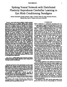
Figure 1. Four typical training data sets – circular classification boundaries in a 2D continuous input space. G1+G1 approach. A more direct second stage strategy involves taking the fitness there to be the number of epochs required to reach the maximum performance level. This we shall call the G1+G2 approach. The next two sections will present a series of simulations which show the levels of performance that arise from the steady state approach (SS) and the three generational approaches (G1, G1+G1, G1+G2), and allow us to identify their respective advantages and disadvantages. These will reveal the unwanted side effects that can emerge from these approaches, and suggest how age dependent plasticity may help.
3. Baseline Simulation Details For concreteness, let us assume that we want to build neural networks that can learn to generalize well on classification tasks, in particular, classifications over unit two dimensional input spaces with random circular classification boundaries. Figure 1 shows some representative cases this covers. Though simplified, such data covers the essential features and difficulties of many real world problems. Each neural network is expected to learn a particular randomly chosen classification boundary from a stream of randomly drawn input data samples. The natural measure of each network’s task performance at each stage is the average number of correct outputs (e.g. within 0.2 of the binary targets) before training on them. For the purposes of computing average performance levels, and updating the steady state populations, it is convenient to separate the training data presentations into blocks of 1200 patterns and call each block a ‘simulated year of experience’. For ease of computation, we shall take our neural networks to be traditional multi-layer perceptrons with one hidden layer, sigmoidal processing units, trained by gradient descent using the cross-entropy error measure. As previous studies have shown [3], it is appropriate to evolve separate learning rates ηL and initial weight distributions [-rL, +r L] for each of the four distinct network components L (the input to hidden weights IH, the hidden unit biases HB, the hidden to output weights HO, and the output unit
biases OB). With standard momentum and weight decay parameters, this gives ten evolvable innate parameters for each network. We could also evolve the number of hidden units, but this invariably results in the maximum number allowed, which slows down the simulations considerably, so we keep this fixed at 20 for all networks, which is plenty for the given task. There remain a number of evolutionary parameters to specify. For the steady state simulations, after each simulated year 10% of the least fit individuals are selected by pair-wise fitness comparisons and removed from the population. Also, to prevent the populations from being dominated by a few very old and very fit individuals, a random 20% of individuals over the age of 30 simulated years are removed each year. In the generational approaches, the least fit 50% of the population are removed at each generation, which for the G1 stages corresponds to 60 simulated years. A fixed population size of 200 is used throughout, with the removed individuals being replaced by children generated from random pairs of the most fit individuals. Innate parameter values for each child are inherited randomly from the corresponding ranges spanned by its two parents, plus random mutations (from a Gaussian distribution) that allows them to fall outside their parents’ ranges.
4. Baseline Simulation Results We can now generate random initial populations and run the evolutionary simulations as described above. Figure 2 shows the evolution of the average learning rates for the four evolutionary approaches, with the standard deviations of the population averages across 10 runs. We can see that the four approaches settle down over rather different evolutionary timescales, and that the final evolved parameters are similar, but significantly different. There are enormous differences in the learning rates that emerge for the different parts of the network, and from the values traditionally used with hand crafted networks. If we evolve a single learning rate for all four components, it comes out at around 0.2 which is in line with traditional values. The evolved initial
10 4
10 4
10 3
etaHO
10 2 10 1
10 3
etaHO
10 2 10 1
etaOB
10 0 10 - 1
etaOB
10 0 10 - 1
etaHB
10 - 2
etaIH
10 - 3 10 - 4
10 - 2
etaHB
10 - 3
etaIH
10 - 4 0
60000
Year
120000
180000
10 4
0
120000
Year
240000
360000
10 4
10 3
10 3
etaHO
10 2 10 1
etaOB
10 0 10 - 1
etaHO
10 2 10 1
etaOB
10 0 10 - 1
etaHB
10 - 2 10 - 3
etaIH
10 - 4 0
60000
Year
120000
180000
etaHB
10 - 2 10 - 3
etaIH
10 - 4 0
60000
Year
120000
180000
Figure 2. Evolution of the neural network learning rates, with means and standard deviations over 10 runs, for the four evolutionary approaches: SS (top left), G1 (top right), G1+G1 (bottom left), G1+G2 (bottom right). weight distributions also exhibit large differences across components, and from the traditional values. The distributions for the initial input to hidden weights and the biases take on well defined values, but for the hidden to output weights we find much wider variations within and across runs, which is a consequence of their relatively minor effect on final performance. The momentum and weight decay parameters invariably take on such low values that their effect is negligible, as one would expect given the way the stream of training data is drawn randomly from a continuous distribution. In this study it is the performance levels of the evolved populations that we are primarily interested in. To provide a statistically reliable measure, the evolved individuals were each tested on 100 different random data distributions. The means and variances of the error rates during learning are plotted in Figure 3. The relatively high error values and standard deviations for the steady state and two stage generational approaches, compared with the single stage G 1 generational approach, suggest significant tails at the high end of the error distributions. This is confirmed by Figure 4
which shows the average error distributions for trained evolved networks between the ages 50 and 60. All four evolved populations have massive peaks at zero errors, as one would hope, but there remain surprising numbers of very large errors. Only the G1 approach manages to be fairly free of such problems. By comparison, most evolved networks with only a single learning rate will still not have fully learned the task by age 60, but there are very few that exhibit very large errors beyond age 50. To understand the differences between the evolved populations for the four approaches, we need to consider the different evolutionary pressures involved. The G1 approach only has the performance at age 60 driving the evolution, and consequently it ends up with the best performance at that age. It has nothing to directly encourage fast learning, so we might expect it to be slower to learn at earlier ages, but in fact it does not end up that much slower than the other approaches. The G1+G1 approach measures the fitness as the average performance over an increasing number of years prior to age 60, which will naturally improve the rate at which most individuals learn, but this also
100
Std.Dev.
100
10
Errors
1 eta
G1+G2
Errors
G1+G2
1
SS
10
SS
G1+G1
G1+G1
1 eta
G1
G1
.1
1 0
20
Age
40
60
0
20
Age
40
60
Figure 3. The errors during learning for the evolved networks: means (left) and variances (right). The four evolved populations are shown (SS, G1, G1+G1, G1+G2), plus a single learning rate G1 population (1 eta) for comparison. 10 0
30
G1+G2
SS
1 eta
20
SS
-5
10 - 1
x 10
10 - 2
1 0 10 - 3
G1+G2
G1 G1+G1
10 - 4 0
2
G1
Errors
4
6
G1+G1
1 eta
0 0
30
Errors
60
90
Figure 4. The error distributions for trained evolved networks: peaks (left) and tails (right). The four evolved populations are shown (SS, G1, G1+G1, G1+G2), plus a single learning rate G1 population (1 eta) for comparison. indirectly encourages a more risky learning strategy with some individuals occasionally failing to learn properly at all, leaving large errors at all ages. The G1+G2 approach encourages fast learning even more directly, by measuring the fitness as the number of epochs required to reach zero errors, and this does lead to even faster learning, but with even more high error instances as a result. Finally, the S S approach encourages faster learning at all ages, resulting in better learning again, but even more of the problematic high error cases. Often one may be able to tolerate occasional very poor performance in return for faster learning most of the time, or faster learning on average. Certainly, in natural systems it can be a good strategy overall for individuals to respond as quickly as possible, even if it leads to occasional deaths. This will be particularly true if it allows more children to be produced before an untimely death than would otherwise be possible in a
full lifetime. On the other hand, if we are using evolution to design a single autonomous system, such a strategy would be unacceptably foolhardy.
5. Age Dependent Plasticity It seems likely, given the lack of problems with the slower single learning rate and G1 networks, that it is the relatively large evolved learning rates that are at the root of the problems with the faster learning populations. It is well known that, for many human abilities, there are critical periods for learning, with high learning rates initially, but much lower rates at older ages (e.g. [4, 5]). More sophisticated learning rate adaptation has also previously proved beneficial for computational systems (e.g. [6]). The idea here is that by allowing learning rates that can vary with age, it may be possible to evolve higher learning rates and faster learning at early ages, whilst having lower
10 4
1.0
10 3 10 2
0.8
10 0
SS
0.6
etaHO
10 1
G1+G2
0.4
etaOB
10 - 1
G1+G1
10 - 2
G1
etaHB
10 - 3 10 - 4
0.2
etaIH
10 - 5 10 - 6
0.0 0
20
Age
40
60
0
20
Age
40
60
Figure 5. The evolved age dependent learning rate scale factors for the four evolutionary approaches (left), and the actual learning rates compared with the corresponding constant learning rates for the SS case (right). 10
Std. Dev.
10
Errors
1
SS
1
G1+G2
Errors
G1+G2
.1
SS
G1+G1
G1+G1 G1
G1 .01
.1 0
20
Age
40
60
0
20
Age
40
60
Figure 6. The error rates during learning for the evolved age dependent plasticity networks: means (left) and variances (right). Population averages from the four evolutionary approaches are shown (SS, G1, G1+G1, G1+G2).
learning rates later and less chance of large errors persisting to older ages. We can simulate such an age dependence by using a simple two parameter exponential scale factor:
η L (t) = s(t) η L (0) , s(t) = β + (1− β ) e −t / τ in which the baseline β and the time constant τ can evolve to take on any positive values. It is then relatively straightforward to repeat all the above simulations with everything else the same, apart from the insertion of this scale factor and its two evolvable parameters. The resulting evolved scale factors, with variances across 10 populations of 200 individuals, are shown on the left of Figure 5. As one might expect, the relatively problem free G 1 populations have a noticeably slower fall off of learning rates with age than the other populations. On the right of Figure 5 is
shown how, for the SS populations, the age dependent learning rates compare with the fixed learning rates we had before. We see that the initial learning rates have adjusted themselves by different amounts to take advantage of the age dependent scaling. Not surprisingly, given the rather different emergent scale factors, the evolved adjustments vary with approach, which means that we no longer have the similarity we saw in Figure 2 between the learning rates across the four evolutionary approaches, and this in turn leads on to somewhat different learning performances. The mean error rates and standard deviations during learning are shown in Figure 6. The first thing to note is the ten-fold scale reduction compared with the corresponding Figure 4, so there is a clear overall improvement. The G1 populations, whose evolution is only driven by final performance, not surprisingly end up with a much improved final performance at age 60, but the initial rate of learning, which was
10 0
0 3
10 - 1
G1
10 - 2
2 0 -5
G1+G1
x 10
10 - 3
SS 10 - 4
G1+G2
1 0
G1+G2
SS
G1+G1
10 - 5
G1
10 - 6
0 0
2
Errors
4
6
0
30
Errors
60
90
Figure 7. The error distributions for trained evolved age dependent plasticity networks: peaks (left) and tails (right). Population averages from the four evolutionary approaches are shown (SS, G1, G1+G1, G1+G2). previously comparable to the evolved fast learners, is now significantly poorer. The G1+G1 populations, which are evolved to have good performance for as many years prior to age 60 as possible, now have a much lower and consistent error rate across those final years, but the earlier reductions in errors are slower. The SS and G1+G2 populations, which are evolved to reduce their error rates as quickly as possible, do now learn much more quickly, but suffer from more cases where there are persistent small errors that are not eliminated by age 60. We see that a consequence of the inherent trade-offs is that evolving improvement in one aspect leads to degradation of others. We have clearly achieved overall lower average error rates by allowing age dependent plasticity, but have we achieved the main objective of reducing the occasional problematic high error cases? Figure 7 shows the error distributions for the trained evolved networks for comparison with Figure 4. The peaks now show much wider variation between evolutionary approaches than before, with the widths of the peaks in proportion to how much the learning speed is taken into account in the evolutionary fitness evaluation. However, all the average error rates are low, and none are significantly worse than we had without the age dependent plasticity, so no new problems have been introduced. In the tails, all four approaches show the hoped for massive reduction in the numbers of very large errors. Naturally, deciding whether that level of reduction is sufficient will be rather problem dependent, but we do now have a much clearer picture of how the different factors interact within the various evolutionary approaches, and what the trade-offs are.
6. Conclusions In this paper we have investigated four natural approaches for evolving neural networks that learn to
classify as well as they can as quickly as they can. Such systems are likely to be a crucial component of a wide range of neural network based autonomous agent applications. The four evolutionary approaches differ in the manner in which the various fitness measures drive the evolution. The more we force faster learning, the riskier the learning strategies that emerge, and the greater the chance of very poor performance. The main aim of this paper was to show how the incorporation of age dependent plasticities could reduce the risk of occasional very poor performance. This reduction was clear, for all four evolutionary approaches, but it also affected the learning speeds, not always for the better. This study has considered the various possibilities, and provides the necessary information for making better informed design decisions in the future.
References [1] X. Yao (1999). Evolving Artificial Neural Networks. Proceedings of the IEEE, 87, 1423-1447. [2] J.A. Bullinaria (2004). Generational versus SteadyState Evolution for Optimizing Neural Network Learning. In: Proceedings of the International Joint Conference on Neural Networks (IJCNN 2004), 22972302. IEEE. [3] J.A. Bullinaria (2003). Evolving Efficient Learning Algorithms for Binary Mappings. Neural Networks, 16, 793-800. [4] B. Julesz and I. Kovacs (Eds) (1995). Maturational Windows and Adult Cortical Plasticity. Reading, MA: Addison-Wesley. [5] D.B Bailey, J.T. Bruer, F. Symons and J.W Lichtman. (Eds) (2000). Critical Thinking About Critical Periods. Baltimore: Brookes. [6] R.A. Jacobs (1988). Increased Rates Of Convergence Through Learning Rate Adaptation. Neural Networks, 1, 295-307.