Evolving Connectionist Systems for On-line, Knowledge-based Learning: Principles and Applications 1 Nikola Kasabov Department of Information Science University of Otago, P.O Box 56, Dunedin, New Zealand Phone: +64 3 479 8319, fax: +64 3 479 8311
[email protected] Abstract. The paper introduces evolving connectionist systems (ECOS) as an effective approach to building on-line, adaptive intelligent systems. ECOS evolve through incremental, hybrid (supervised/unsupervised), on-line learning. They can accommodate new input data, including new features, new classes, etc. through local element tuning. New connections and new neurons are created during the operation of the system. The ECOS framework is presented and illustrated on a particular type of evolving neural networks - evolving fuzzy neural networks (EFuNNs). EFuNNs can learn spatial-temporal sequences in an adaptive way, through one pass learning. Rules can be inserted and extracted at any time of the system operation. The characteristics of ECOS and EFuNNs are illustrated on several case studies that include: adaptive pattern classification; adaptive, phoneme-based spoken language recognition; adaptive dynamic time-series prediction; intelligent agents. Key words: evolving connectionist systems; evolving fuzzy neural networks; on-line learning; spatial-temporal adaptation; adaptive speech recognition. 1. Introduction The complexity and dynamics of real-world problems, especially in engineering and manufacturing, require sophisticated methods and tools for building on-line, adaptive intelligent systems (IS). Such systems should be able to grow as they operate, to update their knowledge and refine the model through interaction with the environment. This is especially crucial when solving AI problems such as adaptive speech and image recognition, multi-modal information processing, adaptive prediction, adaptive on-line control, intelligent agents on the WWW. Seven major requirements of the present IS (that are addressed in the ECOS framework presented later) are listed below [2,35,36,38]: (1) IS should learn fast from a large amount of data (using fast training, e.g. one-pass training). (2) IS should be able to adapt incrementally in both real time, and in an on-line mode, where new data is accommodated as they become available. The system should tolerate and accommodate imprecise and uncertain facts or knowledge and refine its knowledge. (3) IS should have an open structure where new features (relevant to the task) can be introduced at a later stage of the system’s operation. IS should dynamically create new modules, new inputs and outputs, new connections and nodes. That should occur either in a supervised, or in an unsupervised mode, using one modality or another, accommodating data, heuristic rules, text, images, etc. (4) IS should be memory-based, i.e. they should keep a reasonable track of information that has been used in the past and be able to retrieve some of it for the purpose of inner refinement, or for answering an external query. (5) IS should improve continuously (possibly in a life–long mode) through active interaction with other IS and with the environment they operate in.
1
Technical Report 99/02 Department of Information Science, University of Otago, P.O.Box 56, Dunedin, New Zealand. Submitted to IEEE Systems, Man, and Cybernetics, 8 March 1999
1
(6) IS should be able to analyse themselves in terms of behaviour, global error and success; to explain what has been learned; to make decisions about its own improvement; to manifest introspection. (7) IS should adequately represent space and time in their different scales; should have parameters to represent such concepts as spatial distance, short-term and long-term memory, age, forgetting, etc. Unless the above seven issues are addressed in the current and the future IS, it is unlikely that a significant progress is made in areas, such as adaptive speech recognition and language acquisition, adaptive intelligent prediction and control systems, intelligent agent systems, mobile robots, visual monitoring systems, multi-modal information processing, and many more. Several investigations [18,28,43,55,65,66,67,69,74] proved that the most popular neural network models and algorithms are not suitable for adaptive, on-line learning, that includes multilayer perceptrons trained with the backpropagation algorithm, radial basis function networks [58], selforganising maps SOMs [47,48] and these NN models were not designed for on-line learning in the first instance. At same time some of the seven issues above have been acknowledged and addressed in the development of several NN models for adaptive learning and for structure and knowledge manipulation as discussed below. Adaptive learning is aiming at solving the well-known stability/plasticity dilemma [3,4,7,8,9,13,47,48]. Several methods for adaptive learning are related to the work presented here, namely incremental learning, lifelong learning, on-line learning. Incremental learning is the ability of a NN to learn new data without destroying (or at least fully destroying) the learned patterns from old data, and without a need to be trained on the whole old and new data. Significant progress in incremental learning has been achieved due to the Adaptive Resonance Theory (ART) [7,8,9] and its various models, that include unsupervised models (ART1, ART2, FuzzyART) and supervised versions (ARTMAP, Fuzzy ARTMAP- FAM). Lifelong learning is concerned with the ability of a system to learn during its entire existence in a changing environment [82, 69,35,36]. Growing, as well as pruning operation, are involved in the learning process. On-line learning is concerned with learning data as the system operates (usually in a real time) and the data might exist only for a short time. NN models for on-line learning are introduced and studied in [1,2,4,7,11,17,22,28,31,35,36,42,44,46,53,69]. The issue of NN structure, the bias/variance dilemma, has been acknowledged by several authors [6,7,13,65,68]. The dilemma is concerned with the situation where if the structure of a NN is too small, the NN is biased to certain patterns, and if the NN structure is too large there are too many variances that result in over-training, and poor generalisation, etc. In order to avoid this problem, a NN (or an IS) structure should dynamically adjust during the learning process to better represent the patterns in the data from a changing environment. Three approaches have been taken so far for the purpose of creating dynamic IS structures: constructivism, selectivism, and a hybrid approach. Constructivism is concerned with developing NNs that have a simple initial structure and grow during its operation through insertion of new nodes and new connections when new data items arrive. This approach can also be implemented with the use of an initial set of neurons that are sparsely connected and that become more and more wired with the incoming data [62,73,15,19]. The latter implementation is supported by biological facts [62,73,77]. Node insertion can be controlled by either a similarity measure, or by the output error measure, or by both. There are other methods that insert nodes based on the evaluation of the local error, e.g. the Growing Cell Structure, Growing Neural Gas, Dynamic Cell Structure [19,11,13]. Other methods insert nodes based on a global error evaluation of the performance of the whole NN. Such method is the CascadeCorrelation [15]. Methods that use both similarity and output error for node insertion are used in Fuzzy ARTMAP [9]. Cellular automata systems have also been used to implement the constructivist approach [11,4]. These systems grow by creating connections between neighbouring cells in a regular cellular structure. Simple rules, embodied in the cells, are used to achieve the growing effect. Unfortunately in most of the implementations the rules for growing do not change during the evolving process. This limits the adaptation of the growing structure. The brain-building system is an example of this class [11]. 2
Selectivism is concerned with pruning unnecessary connections in a NN that starts its learning with many, in most cases redundant, connections [26,29, 49,56,59,64]. Pruning connections that do not contribute to the performance of the system can be done by using several methods, e.g.: optimalbrain damage [50]; optimal brain surgeon [26]; structural learning with forgetting [29,49]; trainingand-zeroing [32]; regular pruning [56]. Genetic algorithms (GA) and other evolutionary computation techniques that constitute a heuristic search technique for finding the optimal, or near optimal solution from a solution space, have also been widely applied for optimising a NN structure [20,23,13,39,40,71,79,80]. Unfortunately, most of the evolutionary computation methods developed so far assume that the solution space is compact and bounded, i.e. the evolution takes place within a pre-defined problem space and not in a dynamically changing and open one, therefore not allowing for continuous, on-line adaptation. The GA implementations so far have also been very time-consuming. Some NN models use a hybrid constructivist/selectivist approach [52,61,70]. The framework proposed here also belongs to this group. Some of the above seven issues have also been addressed in the knowledge-based neural networks (KBNN) [24,33,38, 63,76,83] as knowledge is the essence of what an IS system has learned. KBNN have operations to deal with both data and knowledge, that include learning from data, rule insertion, rule extraction, adaptation and reasoning. KBNN have been developed mainly as a combination of symbolic AI systems and NN [24, 30,76], or as a combination of fuzzy logic systems and NN [25,30,33,38,39,44,45,51,63,83], or as a combination of a statistical technique and NN [2,4,12,57]. It is clear that in order to fulfil the seven major requirements of the current IS, radically different methods and systems are essential in both learning algorithms and structure development. A framework called ECOS (Evolving COnnectionist Systems) that addresses all seven issues above is introduced in the paper, along with a method of training called ECO training. The major principles of ECOS are presented in section 2. The principles of ECOS are applied in section 3 to develop evolving fuzzy neural network model called EFuNN. Several learning strategies of ECOS and EFuNNs are introduced in section 3. In section 4 ECOS and EFuNNs are illustrated on several case study problems of adaptive phoneme recognition, dynamic time series prediction, and intelligent agents. Section 5 suggests directions for further development of ECOS.
2. The ECOS framework Evolving connectionist systems (ECOS) are systems that evolve in time through interaction with the environment. They have some (genetically) pre-defined parameters (knowledge) but they also learn and adapt as they operate. In contrast with the evolutionary systems they do not necessarily create copies of individuals and select the best ones for the future. They emerge, evolve, develop, unfold through innateness and learning, and through changing their structure in order to better represent data [14,31,35,36]. ECOS learn in an on-line and a knowledge–based mode, so they can accommodate any new incoming data from a data stream, and the learning process can be expressed as a process of rule manipulation. A block diagram of the ECOS framework is given in fig.1. ECOS are multi-level, multi-modular structures where many neural network modules (denoted as NNM) are connected with inter-, and intra- connections. ECOS do not have a clear multi-layer structure, but rather a modular, “open” structure.
3
Action Part
Adaptation
NNM Inputs
• • • New Inputs
Decision Part
NNM
Environment (Critique)
Higher Level Decis. Module
Action Module
Feature Selection Part
Presentation & Representation Part
Results
NNM
Self analysis, Rule extraction
Fig.1 Block diagram of the ECOS framework. The main parts of ECOS are described below. (1) Feature selection part. It performs filtering of the input information, feature extraction and forming the input vectors. The number of inputs (features) can vary from example to example from the input data stream fed to the ECOS. (2) Presentation and representation (memory) part, where information (patterns) are stored. It is a multi-modular, evolving structure of NNM organised in spatially distributed groups; for example one module can represent the phonemes in a spoken language (one NN representing one class phoneme). (3) Higher-level decision part that consists of several modules, each taking decision on a particular problem (e.g., phoneme, word, concept). The modules receive feedback from the environment and make decisions about the functioning and the adaptation of the whole ECOS. (4) Action modules, that take the output from the decision modules and pass output information to the environment. (5) Self-analysis, and rule extraction modules. This part extracts compressed abstract information from the representation modules and from the decision modules in different forms of rules, abstract associations, etc. Initially an ECOS has a pre-defined structure of some NNMs, each of them being a mesh of nodes (neurons) and very few connections defined through prior knowledge, or “genetic” information. Gradually, the system becomes more and more “wired” through self-organisation, and through creation of new NNM and new connections. The ECOS functioning is based on the following general principles: (1) ECOS evolve incrementally in an on-line, hybrid, adaptive supervised/unsupervised mode through accommodating more and more examples when they become known from a continuous 4
input data stream. During the operation of ECOS the higher-level decision module may activate an adaptation process through the adaptation module. (2) ECOS are memory-based and store exemplars (prototypes, rules) that represent groups of data from the data stream. New input vectors are stored in the NNMs based on their similarity to previously stored data both on the input and the desired output information. A node in an NNM is created and designated to represent an individual example if it is significantly different from the previously used examples (with a level of differentiation set through dynamic parameters). Learning is based on locally tuned elements from the ECOS structure thus making the learning process fast for real-time parallel implementation. Three ways to implement local learning in a connectionist structure are presented in [6,7, 47,58]. (3) There are three levels at which ECOS are functionally and structurally defined: (a) Parameter (gene) level, i.e. a chromosome contains genes that represent certain parameters of the whole systems, such as: type of the structure (connections) that will be evolved; learning rate; forgetting rate; size of a NNM; NNM specialisation, thresholds that define similarity; error rate that is tolerated, and many more. The values of the genes are relatively stable, but can be changed through genetic operations, such as mutation of a gene, deletion and insertion of genes that are triggered by the self analysis module as a result of the overall performance of the ECOS. (b) Representation (synaptic) level, that is the information contained in the connections of the NNM. This is the long-term memory of the system where exemplars of data are stored. They can be either retrieved to answer an external query, or can be used for internal ECOS refinement. (c) Behavioural (neuronal activation) level, that is the short-term activation patterns triggered by input stimuli. This level defines how well the system is functioning in the end. (4) ECOS evolve through learning (growing), forgetting (pruning), and aggregation, that are both defined at a genetic level and adapted during the learning process. ECOS allow for: creating/connecting neurons; removing neurons and their corresponding connections that are not actively involved in the functioning of the system thus making space for new input patterns to be learned; aggregating nodes into bigger-cluster nodes. (5) There are two global modes of learning in ECOS: (a) Active learning - learning is performed when a stimulus (input pattern) is presented and kept active. (b) Passive (inner, ECO) learning mode - learning is performed when there is no input pattern presented to the ECOS. In this case the process of further elaboration of the connections in ECOS is done in a passive learning phase, when existing connections, that store previously fed input patterns, are used as “echo” (here denoted as ECO) to reiterate the learning process (see for example fig.9 explained later). There are two types of ECO training: • cascade eco-training: a new connectionist structure (a NN) is created in an on-line mode when conceptually new data (e.g., a new class data) is presented. The NN is trained on the positive examples of this class, on the negative examples from the following incoming data, and on the negative examples from previously stored patterns in previously created modules. • ’sleep’ eco-training: NNs are created with the use of only partial information from the input stream (e.g., positive class examples only). Then the NNs are trained and refined on the stored patterns (exemplars) in other NNs and NNMs (e.g., as negative class examples). (6) ECOS provide explanation information extracted from the NNMs through the self-analysis/ rule extraction module. Generally speaking, ECOS learn and store knowledge, rules, rather than individual examples or meaningless numbers. (7) The ECOS principles above are based on some biological facts and biological principles (see for example [31,55,62,68,72,82]). Implementing the ECOS framework and the NNM from it requires connectionist models that comply with the ECOS principles. One of them, called evolving fuzzy neural network (EFuNN) is presented in the next section.
5
3. Evolving Fuzzy Neural Networks EFuNNs 3.1. General principles of EFuNNs Fuzzy neural networks are connectionist structures that implement fuzzy rules and fuzzy inference [25,51,63,83,38]. FuNNs represent a class of them [38,33,39,40]. EFuNNs are FuNNs that evolve according to the ECOS principles. EFuNNs were introduced in [31,35,36] where preliminary results were given. Here EFuNNs are further developed. EFuNNs have a five-layer structure, similar to the structure of FuNNs (fig.2a). But here nodes and connections are created/connected as data examples are presented. An optional short-term memory layer can be used through a feedback connection from the rule (also called, case) node layer (see fig.2b). The layer of feedback connections could be used if temporal relationships between input data are to be memorised structurally. rule(case) nodes
output
inputs
Fig.2a The five layers basic structure of the EfuNNs.
Outputs
W4
inda1(t )
A1
Fuzzy outputs W2 (t) Rule (base) layer
A1(t-1)
W1
inda1(t-1) W0 W3
x1
x2
Fuzzy input layer Input layer
Inputs
Fig2b EFuNN with a short term memory and a feedback connection
6
The input layer represents input variables. The second layer of nodes (fuzzy input neurons, or fuzzy inputs) represents fuzzy quantization of each input variable space. For example, two fuzzy input neurons can be used to represent "small" and "large" fuzzy values. Different membership functions (MF) can be attached to these neurons (triangular, Gaussian, etc.) (see fig.3).
µ (membership degree)
1 Sthr
The local normalised fuzzy distance
d1f = (0, 0, 1, 0, 0, 0) d2f = (0, 1, 0, 0, 0, 0)
d4
d2
d1
d3
d5
x
Dist(d1d2) = D(d1d3) = D(d1d5) =1
Fig.3. Membership functions (MF) and the local, normalised, fuzzy distance function
The number and the type of MF can be dynamically modified in an EFuNN which is explained later in section 3. New neurons can evolve in this layer if, for a given input vector, the corresponding variable value does not belong to any of the existing MF to a degree greater than a membership threshold. A new fuzzy input neuron, or an input neuron, can be created during the adaptation phase of an EFuNN (see fig.10a,b and the explanation in section 3). The task of the fuzzy input nodes is to transfer the input values into membership degrees to which they belong to the MF. The third layer contains rule (case) nodes that evolve through supervised/unsupervised learning. The rule nodes represent prototypes (exemplars, clusters) of input-output data associations, graphically represented as an association of hyper-spheres from the fuzzy input and fuzzy output spaces. Each rule node r is defined by two vectors of connection weights – W1(r) and W2(r), the latter being adjusted through supervised learning based on the output error, and the former being adjusted through unsupervised learning based on similarity measure within a local area of the problem space. The fourth layer of neurons represents fuzzy quantization for the output variables, similar to the input fuzzy neurons representation. The fifth layer represents the real values for the output variables. The evolving process can be based on two assumptions: (1) no rule nodes exist prior to learning and all of them are created (generated) during the evolving process; or (2) there is an initial set of rule nodes that are not connected to the input and output nodes and become connected through the learning (evolving) process. The latter case is more biologically plausible [82]. The EFuNN evolving algorithm presented in the next section does not make a difference between these two cases. Each rule node, e.g. rj, represents an association between a hyper-sphere from the fuzzy input space and a hyper-sphere from the fuzzy output space (see fig.4a), the W1(rj) connection weights representing the co-ordinates of the center of the sphere in the fuzzy input space, and the W2 (rj) – the co-ordinates in the fuzzy output space. The radius of an input hyper-sphere of a rule node is defined as (1- Sthr), where Sthr is the sensitivity threshold parameter defining the minimum activation of a rule node (e.g., r1, previously evolved to represent a data point (Xd1,Yd1)) to an 7
input vector (e.g., (Xd2,Yd2)) in order for the new input vector to be associated with this rule node. Two pairs of fuzzy input-output data vectors d1=(Xd1,Yd1) and d2=(Xd2,Yd2) will be allocated to the first rule node r1 if they fall into the r1 input sphere and in the r1 output sphere, i.e. the local normalised fuzzy difference between Xd1 and Xd2 is smaller than the radius r and the local normalised fuzzy difference between Yd1 and Yd2 is smaller than an error threshold Errthr. The local normalised fuzzy difference between two fuzzy membership vectors d1f and d2f that represent the membership degrees to which two real values d1 and d2 data belong to the pre-defined MF, are calculated as D(d1f,d2f) = sum(abs(d1f - d2f))/sum(d1f + d2f)). For example, if d1f=(0,0,1,0,0,0) and d2f=(0,1,0,0,0,0) (see fig.3), than D(d1,d2) = (1+1)/2=1 which is the maximum value for the local normalised fuzzy difference . If data example d1 = (Xd1,Yd1), where Xd1 and Xd2 are correspondingly the input and the output fuzzy membership degree vectors, and the data example is associated with a rule node r1 with a centre r11, than a new data point d2=(Xd2,Yd2), that is within the shaded area as shown in fig.3 and fig.4a, will be associated with this rule node too. Through the process of associating (learning) of new data points to a rule node, the centres of this node hyper-spheres adjust in the fuzzy input space depending on a learning rate lrn1, and in the fuzzy output space depending on a learning rate lr2, as it is shown in fig.4a on the two data points d1 and d2. The adjustment of the centre r11 to its new position r12 can be represented mathematically by the change in the connection weights of the rule node r1 from W1(r11 ) and W2(r11) to W1(r12 ) and W2(r12) according to the following vector operations: W2 (r12 ) = W2(r11) + lr2. Err(Yd1,Yd2). A1(r 11) W1(r12)=W1 (r11) + lr1. Ds (Xd1,Xd2) where: Err(Yd1,Yd2)= Ds(Yd1,Yd2)=Yd1-Yd2 is the signed value rather than the absolute value of the fuzzy difference vector; A1(r11) is the activation of the rule node r11 for the input vector Xd2. The learning process in the fuzzy input space is illustrated in fig.4b on four data points d1,d2,d3 and d4. Fig.4c shows how the centre of the rule node r1 adjusts after learning each new data point when two-pass learning is applied. If lrn1=lrn2=0, once established, the centres of the rules nodes do not move. The idea of dynamic creation of new rule nodes over time for a time series data is graphically illustrated in fig.4d. Errt1lr2 2 r1 r1 Yd2 Yd
r11
Y
r12
lr1 2 r11 r1 Xd2 Xd1
X
r Fig4a Input / Output mapping and learning. 8
Fig.4b
Initial sphere for r1
1 – Sthr r11 d1
d2
r14
d4
The r1 sphere after adopting 4 data points
d3
Fig.4c d1
r11(1)
d4 r14(1) r14(2) d3
d2
Output
r2 r1
r3 r1
r2
Inputs over time Fig.4d Dynamic Creation of new rule nodes over time.
9
While the connection weights from W1 and W2 capture spatial characteristics of the learned data (centres of hyper-spheres), the temporal layer of connection weights W3 from fig.2b captures temporal dependencies between consecutive data examples. If the winning rule node at the moment (t-1) (to which the input data vector at the moment (t-1) was associated) was r1=inda1(t-1), and the winning node at the moment t is r2=inda1(t), then a link between the two nodes is established as follows: W3(r1,r2) (t) = W3(r1,r2) (t-1) + lr3. A1(r1) (t-1) A1(r2)) (t) , (t) where: A1(r) denotes the activation of a rule node r at a time moment (t); lr3 defines the degree to which the EFuNN associates links between rules (clusters, prototypes) that include consecutive data examples (if lr3=0, no temporal associations are learned in an EFuNN structure and the EFuNN from fig.2b becomes the one from fig.2a). The learned temporal associations can be used to support the activation of rule nodes based on temporal, pattern similarity. Here, temporal dependencies are learned through establishing structural links. These dependencies can be further investigated and enhanced through synaptic analysis (at the synaptic memory level) rather than through neuronal activation analysis (at the behavioural level). The ratio spatial-similarity/temporal-correlation can be balanced for different applications through two parameters Ss and Tc such that the activation of a rule node r for a new data example dnew is defined as the following vector operations: A1 (r) = f ( Ss. D(r, dnew) + Tc.W3(r (t-1), r)) where: f is the activation function of the rule node r, D(r, d new) is the normalised fuzzy distance value and r (t-1) is the winning neuron at the previous time moment. Figures 5a,b show a schematic diagram of the process of evolving of four rule nodes and setting the temporal links between them for data taken from consecutive frames of phoneme /e/ data as discussed in section 4. r1 /e/1
Spatial-temporal representation of phoneme /e/ data.
W3(1,2) /e/4 r3 /e/3 /e/5
r2
/e/2
W3(2,3)
r4 /e/6
W3 accounts for the temporal links.
W3(3,4)
Fig.5a Consecutive phoneme data frames cause creation of links between the rule nodes. /e/
/e/ t0
t1
t2
t3
r1 r2
/e/
/e/ /e/
/e/ t4
12msec
/e/ t5
r3
/e/ /e/ /e/ /e/
t6
t7
t8
t9
t10
Mel feature vectors over time phoneme /e/
r4
/e/
84msec Fig.5b Schematic diagram of the raw phoneme data and the points in time of rule node creation. 10
. Several parameters were introduced so far for the purpose of control ling the functioning of an EFuNN. Some more parameters will be introduced later, that will bring the EFuNN parameters to a comparatively large number. In order to achieve a better control of the functioning of an EFuNN structure, the three-level functional hierarchy is used here as defined in section 2 for the ECOS architecture, namely: genetic level, long-term synaptic level, and short- term activation level. At the genetic level, all the EFuNN parameters are defined as genes in a chromosome. These are: (a) structural parameters, e.g.: number of inputs, number of MF for each of the inputs, initial type of rule nodes, maximum number of rule nodes, number of MF for the output variables, number of outputs. (b) functional parameters, e.g.: activation functions of the rule nodes and the fuzzy output nodes (in the experiments below saturated linear functions are used); mode of rule node activation ("oneof-n", or “many-of-n”, depending on how many activation values of rule nodes are propagated to the next level); learning rates lr1,lr2 and lr3; sensitivity threshold Sthr for the rule layer; error threshold Errthr for the output layer; forgetting rate; various pruning strat egies and parameters, as explained in the EFuNN algorithm below. 3.2. The EFuNN learning algorithm The EFuNN algorithm, to evolve EFuNNs from incoming examples, is based on the principles explained in the previous section. It is given below as a procedure of consecutive steps. Matrix operation expressions are used similar to the expressions in a matrix processing language such as MATLAB. 1. Initialise an EFuNN structure with a maximum number of neurons and no (or zero-value) connections. Initial connections may be set through inserting fuzzy rules in the structure [44]. If initially there are no rule (case) nodes connected to the fuzzy input and fuzzy output neurons, then create the first node rn=1 to represent the first example d1 and set its input W1(rn) and output W2(rn) connection weight vectors as follows: : W1(rn)=EX; W2(rn ) = TE, where TE is the fuzzy output vector for the current fuzzy input vector EX. 2. WHILE DO Enter the current example (Xdi,Ydi), EX denoting its fuzzy input vector. If new variables appear in this example, which are absent in the previous examples, create new input and/or output nodes with their corresponding membership functions. 3. Find the local normalised fuzzy distance between the fuzzy input vector EX and the already stored patterns (prototypes, exemplars) in the rule (case) nodes rj=r1,r2,…,rn D(EX, rj)= sum (abs (EX - W1(j) )) / sum (W1(j)+EX) 4. Find the activation A1 (rj) of the rule (case) nodes rj, rj=r1:rn. Here radial basis activation function, or a saturated linear one, can be used, i.e. A1 (rj) = radbas (D(EX, rj)), or A1(rj) = satlin (1 – D(EX, rj)). The former may be appropriate for function approximation tasks, while the latter may be preferred for classification tasks. In case of the feedback variant of an EFuNN, the activation A1(rj) is calculated as: A1 (rj) = radbas (Ss. D(EX, rj) - Tc.W3), or A1(j) = satlin (1 – Ss. D(EX, rj) + Tc.W3) . 5. Update the pruning parameter values for the rule nodes, e.g. age, average activation, as predefined in the EFuNN chromosome. 6. Find all case nodes rj with an activation value A1(rj) above a sensitivity threshold Sthr. 7. If there is no such case node, then using the procedure from step 1 in an unsupervised learning mode ELSE 8. Find the rule node inda1 that has the maximum activation value (e.g., maxa1). 9. (a) in case of "one-of-n" EFuNNs (as it is in [9,27,47]) propagate the activation maxa1 of the rule node inda1 to the fuzzy output neurons: 11
A2 = satlin (A1(inda1) . W2(inda1) (b) in case of "many-of-n" mode, the activation values of all rule nodes that are above an activation threshold of Athr are propagated to the next neuronal layer (this case is not discussed in details here; it has been further developed into a new EFuNN architecture called dynamic, ‘many-of-n’ EFuNN, or DEFuNN [42] ) . 10. Find the winning fuzzy output neuron inda2 and its activation maxa2. 11. Find the desired winning fuzzy output neuron indt2 and its value maxt2. 12. Calculate the fuzzy output error vector: Err=A2 - TE. 13. IF (inda2 is different from indt2) or (D(A2,TE) > Errthr ) ELSE 14. Update: (a) the input, (b) the output, an (c) the temporal connection vectors (if such exist) of the rule node k=inda1 as follows: (a) Ds(EX,W1(k)) =EX-W1(k); W1(k)=W1(k) + lr1.Ds(EX,W1(k)), where lr1 is the learning rate for the first layer; (b) W2(k) = W2 (k) + lr2. Err. maxa1, where lr2 is the learning rate for the second layer; (c) W3(l,k)=W3(l,k)+lr3. A1(k).A1(l) (t-1) , here l is the winning rule neron at the previous time moment (t-1), and A1(l) (t-1) is its activation value kept in the short term memory. 15. Prune rule nodes j and their connections that satisfy the following fuzzy pruning rule to a predefined level: IF (a rule node rj is OLD) AND (average activation A1av(rj) is LOW) and (the density of the neighbouring area of neurons is HIGH or MODERATE (i.e. there are other prototypical nodes that overlap with j in the input-output space; this condition apply only for some strategies of inseting rule nodes as explained in a sub-section below) THEN the probability of pruning node (rj) is HIGH The above pruning rule is fuzzy and it requires that the fuzzy concepts of OLD, HIGH, etc., are defined in advance (as part of the EFuNN’s chromosome). As a partial case, a fixed value can be used, e.g. a node is OLD if it has existed during the evolving of a FuNN from more than 1000 examples. The use of a pruning strategy and the way the values for the pruning parameters are defined, depends on the application task. 16. Aggregate rule nodes, if necessary, into a smaller number of nodes (see the explanation in the following subsection). 17. END of the while loop and the algorithm 18. Repeat steps 2-17 for a second presentation of the same input data or for an ECO training if needed. 3.3. Strategies for locating rule nodes in the rule node space There are different ways to locate rule nodes in an EFuNN rule node space as it is explained here. The type selected depends on the type of the problem the EFuNN is designed to solve. Here some possible strategies are explained as illustrated in fig.6: (a) Simple consecutive allocation strategy, i.e. each newly created rule (case) node is allocated next to the previous and the following ones in a linear fashion. That represents a time order. The following statement is valid if no pruning technique is applied, but aggregation technique instead, to optimise the size of the rule layer: at least one example that was associated with rule node rj was presented to the EFuNN before at least one example that was associated to the rule node (rj+1) (see fig.6a). (b) Pre-clustered location, i.e. for each output fuzzy node (e.g. NO, YES) there is a predefined location where the rule nodes supporting this predefined concept are located. At the center of this area the nodes that fully support this concept (error 0) are placed; every new rule node’s location is defined based on the fuzzy output error and the similarity with other nodes (fig.6b);
12
(c) Nearest activated node insertion strategy, i.e. a new rule node is placed nearest to the highly activated node which activation is still less than the Sthr. A connection between the neighbouring nodes can be established similar to the temporary connections from W3. (d) As in (c) but temporal feedback connections are set as well (see fig.2b and fig.6c). New connections are set that link consecutively activated rule nodes through using the short term memory and the links established through the W3 weight matrix; that will allow for the evolving system to repeat a sequence of data points starting from a certain point and not necessarily from the beginning. (e) The same as above, but in addition, new connections are established between rule nodes from different EFuNN modules that become activated simultaneously (at the same time moment) (fig.6d). This would make it possible for an ECOS to learn a correlation between conceptually different variables, e.g. correlation between speech sound and lip movement. output fuzzy concepts Fig.6a.
output
rule nodes
output Fig.6b
fuzzy concepts
output
rule nodes Fig.6.c output fuzzy concepts
output
rule nodes Fig.6d. \
Fig.6. Different strategies for rule node insertion and connection creation
13
3.4 An example of using the EFuNN algorithm in an EFuNN simulator Here, a small speech data set of 400 phoneme data examples is used to illustrate the EFuNN learning algorithm. 100 examples of each of the four phonemes /I/ (from ‘sit’), /e/ (from ‘get’), /ae/ (from ‘cat’), and /i/ (from ‘see’), which are phonemes 25,26,27 and 31 from the Otago Speech Corpus available from the WWW http://kel.otago.ac.nz/, are extracted from the speech data of two speakers of NZ English (one male and one female, numbers 17 and 21 from the Corpus). Each data example used in the experiment described below consists of 3 time lags of 26-element mel-scale vectors, each representing the speech signal within a time frame of 11.6msec, and an output label giving the phoneme class. The speech data is segmented and processed with the use of a 256-point FFT, Hamming window, overlapping of 50% between the consecutive time frames, each of them being 11.6msec long (see fig.5b). An EFuNN with 78 inputs and 4 outputs was evolved on the 400 data examples and tested on another set. Fig. 7a shows the growth of the number of the rule nodes with the progress of entering data examples for one pass of training and the root mean square error RMSE. Fig.7b shows the activation of the /I/ output of the evolved EFuNN for the phoneme /I/ test data (the first 100 examples belong to /I/ and the rest do not belong to it). The parameter values for the EFuNN parameters (e.g. number of evolved rule nodes rn, learning rates lr1,lr2 and lr3, pruning parameters) are shown on the display of the EFuNN simulator which is available from the WWW: http://divcom.otago.ac.nz/infosci/kel/projects/CBIIS/). 200
150
100
50
0 0
50
100
150
200
250
300
350
400
Fig. 7a shows the growth of the number of the rule nodes with the progress of entering data examples for one pass of training and the root mean square error RMSE.
14
1 0. 8 0. 6 0. 4 0. 2 0 0
5 0
10 0
15 0
20 0
25 0
30 0
35 0
40 0
Fig.7b shows the activation of the /I/ output of the evolved EFuNN for the phoneme /I/ test data
3.5. Learning modes in EFuNN. Rule insertion, rule extraction and aggregation. Different learning, adaptation and optimisation strategies and algorithms can be applied on an EFuNN structure for the purpose of its evolving. These include: • Active learning , e.g. the EFuNN algorithm; • Passive learning (i.e., cascade-eco, and sleep-eco learning) as explained in section 2; • Rule insertion into EFuNNs [44]. EFuNNs are adaptive rule-based systems. Manipulating rules is essential for their operation. This includes rule insertion, rule extraction, and rule adaptation. At any time (phase) of the evolving (learning) process fuzzy or exact rules can be inserted and extracted. Insertion of fuzzy rules is achieved through setting a new rule node rj for each new rule R, such that the connection weights W1(rj) and W2 (rj) of the rule node represent the rule R. For example, the fuzzy rule (IF x1 is Small and x2 is Small THEN y is Small) can be inserted into an EFuNN structure by setting the connections of a new rule node to the fuzzy condition nodes x1- Small and x2- Small and to the fuzzy output node y-Small to a value of 1 each. The rest of the connections are set to a value of zero. Similarly, an exact rule can be inserted into an EFuNN structure, e.g. IF x1 is 3.4 and x2 is 6.7 THEN y is 9.5, but here the membership degrees to which the input values x1=3.4 and x2=6.7, and the output value y=9.5 belong to the corresponding fuzzy values are calculated and attached to the corresponding connection weights. • Rule extraction and aggregation. Each rule node r, which represents a prototype, rule, exemplar from the problem space, can be described by its connection weights W1(r) and W2 (r) that define the 15
association of the two corresponding hyper-spheres from the fuzzy input and the fuzzy output problem spaces. The association is expressed as a fuzzy rule, for example: IF x1 is Small 0.85 and x1 is Medium 0.15 and x2 is Small 0.7 and x2 is Medium 0.3 THEN y is Small 0.2 and y is Large 0.8 The numbers attached to the fuzzy labels denote the degree to which the centers of the input and the output hyper-spheres belong to the respective MF. The process of rule extraction can be performed as aggregation of several rule nodes into a larger hyper-spheres as it is shown in fig.8a and fig.8b on an example of three rule nodes r1, r2 and r3 (only the input space is shown there). For the aggregation of two rule nodes r1 and r2, the following aggregation rule is used [44]: IF (D(W1(r1),W1(r2)) < = Thr1) AND (D(W2(r1),W2(r2))