[5] G.J. Gray, Y. Li, D.J. Murray-Smith and K.C.. Shaman: Nonlinear system modelling using output error estimation of a local model network, Proc. SCS. Summer ...
EVOLVING TRAJETORY CONTROLLER NETWOKS FROM LINEAR APPROXIMATION MODEL NETWORKS Yun Li
Gregory Chong
Centre for Systems & Control, Department of Electronics & Electrical Engineering University of Glasgow, Glasgow, G12 8LT, UK. Y.Li @elec.gla.ac.uk
Centre for Systems & Control, Department of Electronics & Electrical Engineering University of Glasgow, Glasgow, G12 8LT, UK. gregccy (3elec.gla.ac .uk
Abstract- Simple, linear classical controllers are highly popular in industrial applications. However, most controllers have to be tuned and manually re-tuned in a trial and error process at every operating level. This is particularly difficult when the plant to be controlled is significantly nonlinear. The deficiency in localised linearised models associated with ‘Local Model Networks’ has been overcome by the introduction of ‘Linear Approximation Model (LAM) Networks’ [2]. To address this problem and help design of industrial controllers for a wider range of operating trajectory, this paper develops a controller network design technique based upon a LAM network of a practical or nonlinear system to be controlled. This is termed a ‘Trajectory Controller Network (TCN)’, which overcomes the deficiency associated with ‘Local Controller Networks’. Each element of a TCN can be of a simple form, such as PID, and may be obtained directly from a set of step response data at several typical operating levels for fast prototyping. Since plant step response data are often readily available in control engineering practice, such TCNs can be automatically and optimally evolved from these data directly without the need for model identification. The overall controller is co-ordinated and evolved along the entire operating trajectory in the operating envelope, tackling the control problem of practical or nonlinear plants. Evolutionary computation provides global structural search for the network and multi-objective optimisation of the controllers. This novel technique is illustrated and validated through a nonlinear control example.
techniques [ 5 ] have provided some effective solutions to these problems, but they are based on locally linearised models. To address these problems more completely for a wider range of the operating trajectory and to make use of plant step-response data that are often readily available in engineering practice, this paper proposes a trajectory controller network (TCN) technique based on linear approximation model (LAM) technique [ 2 ] . Such a LAM network is obtainable directly from plant step-response data by fitting nonlinear trajectories globally between two operating levels. As preliminaries to design, this modelling technique is outlined in Section 2. Based upon a LAM, each TCN controller node can be obtained in a simple form, such as in the proportional plus integral plus derivative (PID) form, straightforwardly by classical design or evolutionary means. The TCN technique is detailed in Section 3. Section 4 illustrates and validates the technique through a nonlinear control example. Finally, conclusions are drawn in Section 5.
1,Introduction A dynamic engineering system is usually nonlinear and complex in practice. Plant dynamics may vary significantly with changes of operating conditions. Therefore, the use of a single nominal linear model under one operating condition, and hence controllers designed out of such a plant model, are often unreliable and inadequate to represent a practical system. The recently developed local controller network
0-7803-6375-2/00/$10.0002000 IEEE.
25 1
2 Linear Approximation Model for Nonlinear System Modelling 2.1 LAM Technique A LAM approximates step response data by a transfer
function or transfer function matrix. This is similar to represent a nonlinear system response with high fidelity by convolution or harmonic analysis. This simple technique eases the difficulties encountered in conventional linearisation without the need for an initial nonlinear model. Unlike a local model network, LAM gives a straightforward approximation in the entire trajectory ranging from the initial condition to the set point, whilst a local model network is applicable only around the initial condition. To achieve high modelling quality and fast generation of LAM, an evolutionary algorithm may be used to search for globally optimal solutions. For more adaptive ness, further fine-tuning by local optimisation method may be applied. This method is illustrated in Fig. 1.
Gravitational constant
g = 9.81 m s-'
Per-volt Pumo Flow rate
0,= 0.000007(m3s-l v-')
I Flow rate from tank 1 to tank 2 I Ql (m3s-') I
I
1 Q, (m3s-')
Discharge rate
....... .....
:".:..
I
output (h,) versus Inpuqy) 0 18 0 16
-
30 Fig. 1. Evolving a LAM network from plant step response data.
004
2.2 Validation of a LAM Here, the LAM to approximate a nonlinear plant is illustrated through an example. The nonlinear plant used for the example is a twin-tank coupled nonlinear hydraulic system that models liquid-level found in chemical and diary plants. Based on the Bemoulli's mass-balance and flow equations, the system structure is given by equation (1).
hl (m)
h, (m) Minimum height of liquid in tank Ho = 0.03 m c1 = 0.53
Discharge coefficient of orifice 2
c, = 0.63
I Cross sectional area of orifice 1 I ul = 0.0000396 m2 1 Cross sectional area of orifice 7- I U, = 0.0000386 m2
If three operating points on the nonlinear trajectory are used, they can be chosen based on the rate of change or equally divided from the full operating range of the liquid level. The simple division is used because of the trajectory capability of the LAM models. The three operating points used in this test are 0.05m, O.lm and 0.15m. Using the step response from nonlinear model at operating point of O.lm for Tank 2 as an example, an evolved LAM fits the responses of level in Tanks 1 and 2 accurately as shown in Fig. 3, where the corresponding step responses actually overlap on each other.
0251
0
'
Validation of LAM model LAMhl
-Planthl
200
400
600 Time ( 5 )
Planth2
800
LAMh2
1000
1200
Fig. 3. Validation of LAM at operating level O.lm
Height of liquid in tank 2
A =O.Ol m2
Fig. 2. Non-linearity of the plant, where h, is a steady state liquid level against the input voltage v,.I
1
Table 1: Nonlinear system parameters
Discharge coefficient of orifice 1
0 02
I
The system input is the voltage applied to the pump, vi, and the system output is the liquid level in tank 2, h,. The coefficients of the twin tank are tabulated in Table 1. The non-linearity of the plant model is clearly plotted as shown in Fig. 2.
Cross sectional area of tank 1&2
012 01 008
5 006
In modelling a nonlinear system, a set of LAMS obtained at different operating points can be networked conveniently by simple linear local interpolation to produce an unseen operating level if require. Compared with a local model network, a LAM network offers the advantage of obtaining each linear model directly from step response and hence the advantage of wide range of validity of individual models that can act stand-alone in a certain degree.
Height of liquid in tank 1
014
To further validate the LAM network, a set of LAMS was generated at different operating point and the unseen operating points produce from LAM network are shown as dotted line in Fig. 4, where again the modelled responses overlap with the actual data.
I
I
252
Weight
Fig.
Fig. 4. Step responses of a LAM network at seen operating point sand the unseen ones at 0.75m and 0.125m.
3 TCN and Its Evolutionnary Design A simple PID control system can be design easily out of a LAM. To apply the TCN technique to nonlinear plants, controllers are designed for the entire LAM network of the nonlinear system. The network is to provide adequate performance across the operating envelope of the system. For the LAM obtained in the previous section, three PID controllers in the TCN are scheduled or simply switched between them as shown in Fig. 5. During a controller operation, a variable indicating operating point is monitored and different controllers (or controller parameters) are activated according to this scheduling variable. In this design, the plant output y(t) is used as scheduling variable to weight the output of the controllers. In real world most of the actuators have its limit. If a controller with an integrating action is used, the error may continue to be integrated when the actuator saturates, leading to, “wind up”. Therefore, anti-windup is implemented in the TCN developed here.
6. A simple interpolation schedule in forming a TCN
Therefore, at any output level y(t), the individual controller outputs u,(t) are interpolated giving a final controlling output u(t) using equation (2). Fig. 6 shows that the sum of 70% of controller 1 output and 30% of controller 2 output was the control effort to the plant. In this test, P,=0.05m, P,=O.lm and P,=O. 15m.
U(f)
=
I
In equation (2), i=l,...,n-1 and n is the total number of linear controller. Using the same method, interpolation may also applied to the controller parameters K,, K , and K,.
4 Design Example and Validation 4.1 Generating Trajectory Controllers From Step Responses Data Individual PID controllers from a step-response trajectory to each of the three operating points are generated from the PIDeasyTM design package for PID control systems [4], as shown in Fig. 7.
I
e.5.
Y ’ Multiple linear controller based trajectory controller
network.
The TCN can use a simple linear interpolation schedule to weight the controllers as shown in Fig. 6. This combined control effort offers a good global close-loop performance under different operating condition of the nonlinear system is a simple way.
25 3
Fig. 7. Direct design from plant response using PIDeasym
PIDeasyTM analyses step response data and generates an appropriate PID controller from them in a matter of seconds. At each operating point, the step response of the LAM
produces a corresponding PID controller. Individual controller parameters generated are shown in Table 2. Table 2. PID controller parameters generate from linear technique individually.
PID controller
0.5353 At O.lm At 0.15m The closed loop performance at these operating points is plotted on the same graph shown in Fig. 8. Note that here, each PID controller was generated using 'linear' stepresponse data, but now tested against the nonlinear plant. This reveals the need for network tuning. Fig. 9. Objective function for optimising the controller at one reference point.
0.18 0.16 0.14
To evolve the TCN for the entire operating envelope, a few pre-select reference points are used. Therefore, at n reference operating points the overall cost function is given in equation ( 3 ) . Where e(t) is the tracking error.
-p 0.12 0.1
? 0.08 L:
0.06 0.04 0.02 0
(3) 0
I
I
200
400 TI-
I
,
600
800
I
In the GA search, three reference levels are used to evaluate the error tracking performance which are representative to the whole operating trajectory. Each reference is tested for a period of m=1000 sec. The evolved TCN will be use to test against two unseen operating points at 0.075m and 0.125m as shown in Fig. 10.
1000
lac)
Fig. 8. Performance of each individual trajectory PID controller tested against the nonlinear plant at different operating levels including the unseen ones at 0.75mand 0.125m.
4.2. Networking Through Evolution A genetic algorithm (GA) provides globally optimal solutions to engineering design problems by emulating natural evolution [6]. A population of potential solutions evolve using crossover, mutation and selection operators to arise at better and better solutions. One advantage of a GA for search and tuning is that the objective or fitness function needs not to be differentiable. This is useful for global optimisation involving nonlinearity and actuator limits. Here, the objective function to be minimised is the L, norm of all errors across the closed loop response within a given time period m as shown in Fig. 9.
L
L
Operating Ievel
Fig. 10. Evaluation points in the operating envelope.
To evolve a out of LAM, all the parameters of the three linear controllers and the scheduling weights are evolved simultaneously in operating envelope. At the end of 50 generations of a population size of 50, the controller parameters obtained are tabulated in Table 3.
254
Table 3. PID controller parameters generate from linear technique individually.
Bibliography [ l ] G.J. Gray, D.J. Murray Smith, Y. Li, K.C. Shaman, T. ( 1998) “Weinbrenner: Nonlinear model structure identification using genetic programming,” Control Engineering Practice, VoI.6, No.11. 1341-1352. [2] Y. Li and K.C. Tan. (2000) “Linear approximation model network and its formation via evolutionary computation,” Academy Proceedings in Engineering Sciences (SADHANA), Indian Academy of Sciences, June. [3] D.E. Goldberg: (1989) “Genetic Algorithm in Search, Optimisation and Machine Learning,” AddisonWesley, Reading.
PID controller
At 0.15m
213.5472
14.34384
The closed loop responses of the finally evolved TCN are shown in Fig. 11. From the results, it can be seen that the performance excel that of the individually tune method show in Fig. 8. providing a fast optimal solution to the nonlinear control problem. Closed loop responses of TCN
0 18
0.14
Oo2
1 I
-0
15m
i 0
200
400
W O Time(rc)
800
1000
1200
’
Fig. 11. Closed loop responses of the TCN at operating points including the unseen ones at 0.125m and 0.075m.
5 Discussion and Conclusion To provide simple and effective control system design in an operating envelope of a nonlinear plant, this paper has developed a trajectory controller network (TCN) technique based on linear approximation model (LAM)networks. The example shows that a linear TCN offers high performance in the control of a nonlinear system in the entire operating envelope. This tremendously simplifies nonlinear control system design. The results also show that a GA automated controller network design for nonlinear systems is possible and useful and such a network can easily be designed from sampled response data.
Acknowledgments The second author is grateful to University of Glasgow and CVCP for a Postgraduate Scholarship and an ORS Award.
255
[4] Y. Li, W. Feng, K.C. Tan, X.K. Zhu, X. Guan and K.H. Ang. (1 998) “PIDeasyTM and automated generation of optimal PID controllers,” The Third Asia-Pacific Conference on Measurement and Control, Dunhuang, China, Plenary paper, 29-33. [5] G.J. Gray, Y. Li, D.J. Murray-Smith and K.C. Shaman: Nonlinear system modelling using output error estimation of a local model network, Proc. SCS Summer Computer .Simulation Conference, Poland, OR, 460-465, IPP6. [6] G.J. Gray, Y. Li, D.J. Murray-Smith and K.C. Shaman. (1995) “Specification of a control system fitness function using constraints for genetic algorithm based design methods,” Proc. First IEEYIEEE! Int. Conf. on GA in Eng. Syst.: Innovations and Appl., Sheffield, 530-535. [7] Y. Fathi. (1997) ”A linear approximation model for the parameter design problem,” European Journal of Operational Research, Vo1.97, No.3, 561-570. [SI Klatt and Engell. (1998) “Gain-scheduling trajectory control of a continuous stirred tank reactor,” Computers & Chemical Engineering, V01.22, No.4-5, 491-502. [9] G. Coniga, A. Giua, G. Usai. (1998) “An implicit gain-scheduling controller for cranes,” IEEE Trans, Control Systems Technology, V01.6, No.1, 15-20. [lOIGawthrop, P.J., Jezek, J., Jones, R.W. and Sroka, I. (1993) “Grey-box model identification,” Invited Paper, Control-Theory and Advanced Tech., 9, (1j, pp. 139-157. [11]Y. Li, K.C. Tan and M.R. Gong. (1997) “Global structure evolution and local parameter learning for control system model redutions,” Evolutionary Algorithms in Eng. Appl., Dasgupta, D. and Michalewicz, Z. (Eds.), Springer Verlag.