Apr 27, 2004 - scan fan-beam reconstruction (360 degree) or from a short-scan reconstruction. In the latter ... Physically, Ω represents the field-of-view of the scanner. .... n = (−R sinλ + ucos λ, R cos λ + usinλ)/√R2 + u2 s = Ru/√R2 + u2. (10).
Exact and approximate algorithms for helical cone-beam CT Hiroyuki Kudo1 , Thomas Rodet2 , Fr´ed´eric Noo3 , Michel Defrise2 Dept. of Computer Science, Graduate School of Systems and Information Engineering, University of Tsukuba, Japan 2 Dept. of Nuclear Medicine, Vrije Universiteit Brussel, AZ-VUB, B-1090 Brussels, Belgium 3 Dept. of Radiology, University of Utah, Salt-Lake City, Utah. 1
April 27, 2004
Abstract This paper concerns image reconstruction for helical x-ray transmission tomography (CT) with multirow detectors. We introduce two approximate cone-beam (CB) filtered-backprojection (FBP) algorithms of the Feldkamp type, obtained by extending to three dimensions (3D) two recently proposed exact FBP algorithms for 2D fan-beam reconstruction. The new algorithms are similar to the standard Feldkamp-type FBP for helical CT. In particular, they can reconstruct each transaxial slice from data acquired along an arbitrary segment of helix, thereby efficiently exploiting the available data. In contrast with the standard Feldkamp-type algorithm, however, the redundancy weight is applied after filtering, allowing a more efficient numerical implementation. To partially alleviate the CB artefacts, which increase with increasing values of the helical pitch, a frequency-mixing method is proposed. This method reconstructs the high frequency components of the image using the longest possible segment of helix, whereas the low frequencies are reconstructed using a minimal, short-scan, segment of helix to minimize CB artefacts. The performance of the algorithms is illustrated using simulated data.
1
Introduction
This paper concerns the image reconstruction problem for helical x-ray transmission tomography (CT) with multi-row detectors. An exact solution to this problem has been recently introduced by Katsevich (2002, 2002a, 2003) and leads to an efficient filtered-backprojection (FBP) algorithm for the reconstruction of a 3D function from axially truncated cone-beam (CB) projections acquired with a helical path of the x-ray source relative to the patient. In this algorithm, the CB projections are first differentiated with respect to the helical path length; a 1D Hilbert filter is then applied along one or several families of straight lines in the detector, and the filtered CB projections are finally backprojected as in the well-known algorithm of Feldkamp, Davis and Kress (1984). 1
One of the key points in the derivation of Katsevich’s algorithm is the definition of families of filtering lines that guarantee exact reconstruction, allow the handling of axially truncated projections, and efficiently use the available detector area to optimize the signal-tonoise ratio (SNR). To date, families of filtering lines that yield exact reconstruction have been defined only for two specific cases, referred to here for convenience as the PI-reconstruction and the 3 PI-reconstruction. With the PI-reconstruction, each point in the image volume is reconstructed using the segment of helix bounded by the PI-line of the point1 . This is the smallest helix segment compatible with exact reconstruction, and therefore, when the detector size is fixed, the PI-reconstruction allows to maximize the helical pitch. The 3 PIreconstruction reconstructs each point P from a longer segment of helix bounded by a line containing P and two points of the helix with an axial separation comprised between one and two times the pitch. As with the PI reconstruction, however, the 3 PI-reconstruction makes efficient use of the available detector area only for a well defined value of the helical pitch. Thus being restricted to these two specific cases, the exact algorithms known to date do not allow optimal data utilization with arbitrary values of the helical pitch, for a fixed size of the detector. This motivates continuing research on approximate algorithms that can more easily be adapted to general configurations. Two approaches have been proposed so far: • Generalizations (Stierstorfer et al 2002, Tang 2003, Flohr et al 2003) of the advanced single slice rebinning algorithm (Larson et al 1998, Heuscher 1999, Noo et al 1999, Kachelriess et al 2000, Defrise et al 2001, 2003), • Generalizations of the FDK algorithm (Feldkamp et al 1984) for helical data (Kudo and Saito 1992, Wang et al 1993, Yan and Leahy 1992). The second approach will be discussed in this paper. The approximate algorithms of the FDK type are derived by extending to 3D standard algorithms for 2D fan-beam reconstruction. Specifically, an exact 2D fan-beam inversion formula is first written for each point P = (x0 , y0 , z0 ), assuming a virtual circular orbit contained in the transaxial plane z = z0 . The ray-sums required by this 2D fan-beam inversion formula are then replaced by measured ray-sums diverging from locations of the x-ray source along its circular or helical path. The 2D fan-beam backprojection is thereby converted into a 3D cone-beam backprojection, while the ramp filtering remains the same as in the 2D case (the nature of the lines in the detector along which the filter is applied will be discussed below). This strategy has been applied to circular and to helical CT, starting either from a fullscan fan-beam reconstruction (360 degree) or from a short-scan reconstruction. In the latter case, data redundancy is handled using the weighting proposed by Parker (1982). Parker’s weighting for data redundancy, however, can be generalized to arbitrary angular ranges, up to 360 degrees (Silver 2000), and possibly exceeding 360 degrees. Extending the resulting 1
The PI-line of a point P is the unique line through P that connects two points of the helix separated axially by less than one pitch.
2
algorithms to 3D in the same way as for the standard FDK method leads to an approximate CB-CT algorithm in which each point P = (x0 , y0 , z0 ) is reconstructed from a segment of helix centered, axially, at z = z0 . The length of the helix segment is arbitrary, provided it is larger than the short-scan segment and does not exceed the maximum size allowed by the detector size. Besides its approximate nature, the main drawback of the FDK type approach for helical CB-CT is that the cone-beam projections must be filtered more than once (Kudo et al 1999). This property is due to the fact that the projections must be multiplied by Parker’s weight prior to filtering (see Parker 1982 and Wesarg et al 2002). But Parker’s weight depends on the location of the x-ray source relative to the segment of helix used for reconstruction, and since this segment is centered on the transaxial slice z0 , the weight applied to a given detector row depends on the slice z0 to which this row contributes. Therefore, each row must be weighted and then filtered, once for each image slice onto which it is backprojected. This added computational complexity is only avoided when the segment of helix used for reconstruction is an integer multiple of 2π since Parker’s weight is constant in that case. In this paper, we introduce two approximate algorithms for helical CB-CT which can be applied to arbitrary helix segments. These algorithms are obtained by extending to 3D, in the same way as above, two recently discovered 2D fan-beam reconstruction algorithms (Noo et al 2002, Kudo et al 2002) based on a relation between fan-beam projections and parallel-beam projections (Hamaker et al 1980). The main property of these algorithms is that the redundancy weight is applied after filtering. This property allows to filter each projection only once, hence considerably simplifying the extension to helical CT. The paper is organized as follows. After introducing notations in section 2, the two fan-beam FBP algorithms are described in section 3, and are then extended in section 4 to helical CT. The link between the resulting approximate algorithms and exact CB-FBP methods is discussed in section 5, allowing a characterization of the approximation in terms of the 3D Radon transform. The link with the exact methods will also provide some motivation for selecting filtering lines in FDK type algorithms that are parallel to the tangent to the helix, as originally proposed by Yan and Leahy (1992). These results naturally lead to a new algorithm, described in section 6. This algorithm reconstructs the low- and the highfrequency components of the object using respectively a short and a longer helix segment; this technique efficiently exploits the available detector data while minimizing the conebeam artefacts due to the approximate character of the FDK algorithms. Finally, in section 7, results with simulated data illustrate the accuracy of the proposed methods and their potential to reduce image noise by using redundant CB data in an efficient way.
2
The helical CT data and the 3D x-ray transform
Figure 1 illustrates the data acquisition geometry. We use f (~r) with ~r = (x, y, z) to describe the density function to be reconstructed and assume that this function is smooth and vanishes
3
outside the cylinder
n
o
Ω = (x, y, z) ∈ IR3 x2 + y 2 ≤ RF2 OV .
(1)
~a(λ) = (R cos λ, R sin λ, hλ)
(2)
We will write equivalently f (~r) = f (x, y, z). Physically, Ω represents the field-of-view of the scanner. To reconstruct f (~r), we measure CB projections for cone vertices on the helical path ~a(λ) oriented along the z-axis:
where λ ∈ IR is the angle describing the rotation of the cone vertex, R > RF OV is the radius of the helix and P = 2πh is its pitch. In CT, the cone vertex represents the position of the x-ray source relative to the object or patient. As illustrated in figure 1, we consider a flat area detector which moves with the cone vertex. At angular position λ, the detector is parallel to the z-axis and to the vector ~a0 (λ) = d~a(λ)/dλ tangent to the helix. To simplify the derivations, we assume below that the distance from ~a(λ) to the detector is R, i.e. the detector contains the z-axis2 . To locate detector pixels in space, we introduce cartesian coordinates u and v in the plane D(λ) containing the area detector. These coordinates are measured along two orthogonal unit vectors ~1u and ~1v in D(λ), with ~1v parallel to the axis of the helix: ~1u (λ) = (− sin λ, cos λ, 0)
~1v (λ) = (0, 0, 1)
(3)
The origin (u, v) = (0, 0) is at the orthogonal projection of ~a(λ) onto D(λ), and the measured range is (u, v) ∈ [−uD , uD ]×[−vD , vD ]. We assume that the q detector is large enough to avoid truncation along the u axis, so that uD ≥ um = RRF OV / R2 − RF2 OV . The CB projection for vertex position λ is the set of line integrals g(u, v, λ) which connect ~a(λ) to points (u, v) in D(λ): g(λ, u, v) =
p
R2
+
u2
+ v2
Z
l0 (u)+∆l(u)
�
dl f X(λ, u, l), Y (λ, u, l), hλ + lv l0 (u)−∆l(u)
�
(4)
with (u, v) ∈ [−uD , uD ] × [−vD , vD ] and X(λ, u, l) = R cos λ + l(−R cos λ − u sin λ) Y (λ, u, l) = R sin λ + l(−R sin λ + u cos λ)
(5)
The limits of the integral in equation (4) are determined by the intersection of the ray with the boundary of the cylindrical field-of-view Ω: l0 (u) = R2 /(R2 + u2 )
,
∆l(u) =
q
(u2m − u2 )(R2 − RF2 OV )/(R2 + u2 )
(6)
2 Scaling all equations by substituting u → uR/D and v → vR/D is sufficient to describe the case of a plane detector located at a distance D from the vertex.
4
This paper deals with the reconstruction of f (x, y, z) from the cone-beam projections acquired on a helix segment λ ∈ Λ(z) = [z/h − ∆Λ /2, z/h + ∆Λ /2] centered axially on the slice z and having a specified angular range ∆Λ . As outlined in the introduction, approximate solutions to this problem will be defined by first considering in the next section the reconstruction of a transaxial slice z = z0 from its 2D Radon transform.
3
Two-dimensional fan-beam reconstruction with redundant data
The 2D Radon transform of a slice f (x, y)3 will be parametrized using the fan-beam sampling defined by restricting to 2D the 3D geometry of equation (4): g(λ, u) =
p
R 2 + u2
Z
l0 (u)+∆l(u)
�
�
dl f X(λ, u, l), Y (λ, u, l)
l0 (u)−∆l(u)
| u |≤ um , λ ∈ Λ
(7)
These data correspond to a set of ray-sums diverging from locations of the x-ray source along a segment of circle ~a2D (λ) = (R cos λ, R sin λ), λ ∈ Λ = [−∆nΛ /2, +∆Λ /2]. The length ∆Λ of this segment must be such that any line crossing Ω2D = (x, y) ∈ IR2 x2 + y 2 ≤ o
RF2 OV intersects the circle segment at least once (Natterer 1986). This 2D data sufficiency condition is satisfied when the segment is not smaller than the short-scan segment, i.e. when ∆Λ ≥ π + 2 arcsin(RF OV /R). In this paper, however, we consider larger segments which may exceed 2π, even though this makes little sense in a 2D context. In this case, the data are redundant and the number N (λ, u) of intersections between a ray-sum parameterized by (λ, u) and the circle segment is not constant. To account for this redundancy, one introduces a smooth normalization function w(λ, u) such that for any pair (λ ∈ Λ, u ∈ [−um , um ]), N (λ,u)
X
w(λj , uj ) = 1
(8)
j=1
where ~a2D (λj ), j = 1, · · · , N (λ, u) are the intersections of the ray (λ, u) with the circle segment ~a2D (Λ), and uj , j = 1, · · · , N (λ, u) are the corresponding detector coordinates, so that all rays (λj , uj ), j = 1, · · · , N (λ, u) coincide. The simplest normalization function is w(λ, u) = 1/N (λ, u) but differentiable functions are prefered for better numerical stability, and are even required by some algorithms. Starting from the standard FBP algorithm for the inversion of the Radon transform with parallel-beam parameterization, inversion formulae for fan-beam data have been derived by exploiting relations linking the fan-beam data g(λ, u), equation (7), to parallel-beam data p(s, ~n) =
Z
Ω2D
3
d~rf (~r) δ(s − ~n · ~r)
We consider in this section a fixed slice z = 0 and drop the third argument of f .
5
(9)
with the well-known relation between the parallel-beam and fan-beam parameters p
~n = (−R sin λ + u cos λ, R cos λ + u sin λ)/ R2 + u2 p
s = Ru/ R2 + u2
(10)
Three such 2D fan-beam inversion formulae are given below: • FBP-1: Using the direct link p(s, ~n) = g(λ, u), one gets the standard fan-beam FBP (Parker 1982): R2 gF (λ, U (x, y, λ)) (R − x cos λ − y sin λ)2 1
(11)
U (x, y, λ) = R(−x sin λ + y cos λ)/(R − x cos λ − y sin λ)
(12)
f (x, y) =
Z
dλ
Λ
where is such that the ray defined by (λ, U (x, y, λ)) contains the point (x, y). The filtered projections are given by g1F (λ, u0 ) =
Z
um
−um
du hR (u0 − u)w(λ, u) √
where hR (u) is the kernel of the ramp filter, hR (u) =
R g(λ, u) R 2 + u2
R∞
−∞ dν
(13)
|ν| exp(2πiνu).
• FBP-2: Using the relation of Hamaker (1980) between the Hilbert transforms of p(s, ~n) and of g(λ, u), one obtains (Kudo et al 2002): f (x, y) =
Z
dλ
Λ
R2 (R − x cos λ − y sin λ)2
n
+
F w(λ, U ) g2R (λ, U )
o ∂w(λ, u) F g2H (λ, U ) u=U ∂u
(14)
where U = U (x, y, λ) is as in equation (12), and the two filtered fan-beam projections are given by F g2R (λ, u0 )
=
F g2H (λ, u0 ) =
where hH (u) =
R∞
−∞ dν
um
R g(λ, u) + u2 −um Z um 1 R g(λ, u) du hH (u0 − u) √ 2 2π −um R + u2
Z
du hR (u0 − u) √
R2
(15) (16)
(−i) sign(ν) exp(2πiνu) is the kernel of the Hilbert transform.
• FBP-3: Finally, the derivative of Hamaker’s relation with respect to λ leads to a third inversion formula (Noo et al 2002): f (x, y) =
Z
Λ
dλ
1 w(λ, U ) g3F (λ, U ) R − x cos λ − y sin λ 6
(17)
where again U = U (x, y, λ), and g3F (λ, u0 )
1 = 2π
um
R du hH (u − u) √ R 2 + u2 −um
Z
0
∂ R 2 + u2 ∂ + ∂λ R ∂u
!
g(λ, u)
(18)
Note that this last formula involves the first power of the magnification weight in the backprojection. Compared to standard fan-beam FBP, the last two algorithms have two important advantages. The first one is that the exact reconstruction of a point (x, y) requires the normalisation condition (8) to be satisfied only for all rays containing (a neighbourhood of) that point. Therefore, some subset of the FOV Ω2D can be reconstructed from fanbeam data acquired along a segment of circle shorter than the short-scan segment π + 2 arcsin(RF OV /R) (Noo et al 2002). In contrast, the standard fan-beam reconstruction FBP-1 requires measuring all rays through the object, even if only part of the FOV needs to be reconstructed. The length of the circle segment must then be at least a short-scan π + 2 arcsin(RF OV /R). The second property of the algorithms FBP-2 and FBP-3 is that the redundancy weight w(λ, u), or its derivative, is applied after filtering the data, in contrast with the standard fan-beam FBP of equation (13). As will be seen in the next section, this property simplifies the extension to helical cone-beam data.
4
Two new Feldkamp-type algorithms for helical CT
In this section we extend the 2D fan-beam FBP algorithms to reconstruct the helical conebeam data defined by equation (4). This empirical extension follows the same approach as that leading to the classical Feldkamp algorithms (Feldkamp et al 1984). Each transaxial slice z is reconstructed by backprojecting the filtered cone-beam projections acquired on the helix segment Λ(z) = [z/h − ∆Λ /2, z/h + ∆Λ /2] according to equations (11), (14) and (17) for the three fan-beam algorithms respectively. Because we are dealing with cone-beam data g(λ, u, v) instead of fan-beam data g(λ, u), the axial detector variable v must be inserted into these equations. This is done by choosing v in such a way that f (~r) is reconstructed by summing filtered ray-sums containing the point ~r. The filtering of the fan-beam projections in equations (13), (15), (16) and (18) is extended to cone-beam projections with three modifications: √ √ 1. The weighting factors R/ R2 + u2 are replaced by R/ R2 + u2 + v 2 , 2. The derivative ∂/∂λ+ (R2 + u2 )/R ∂/∂u in equation (18) is a derivative with respect to the parameter λ for a fixed direction of the ray. It is replaced in 3D by the corresponding derivative at fixed spatial direction, which is ∂/∂λ + (R2 + u2 )/R ∂/∂u + (uv/R)∂/∂v,
7
3. The direction in the detector along which the ramp and Hilbert filters must be applied is not defined unambiguously when extending empirically the algorithms to 3D. For the usual helical Feldkamp algorithm, the ramp filter has been applied either along the ~1u axis orthogonal to the helix axis z (Kudo and Saito 1992, Wang et al 1993), or along an axis ~1ur rotated by an angle η = arctan(h/R) with respect to the u axis (Yan and Leahy 1992): ~1ur = cos η ~1u + sin η ~1v = (− cos η sin λ, cos η cos λ, sin η)
(19)
This axis ~1ur is parallel to the tangent ~a0 (λ) to the helix at the vertex considered (we omit for simplicity the dependence of these unit vectors on λ). Several studies (Turbell and Danielsson 1999, Sourbelle and Kalender 2003) indicate that filtering along ~1ur instead of ~1u significantly reduces cone-beam artefacts, and this approach will be selected in this paper. We are now ready to define the three Feldkamp-type algorithms: • FDK-1 The standard FDK algorithm is the 3D extension of FBP-1: f (~r) =
Z
dλ
Λ(z)
R2 gF (λ, U, V ) (R − x cos λ − y sin λ)2 1
(20)
where U = U (x, y, λ) as in the previous section and V = V (x, y, z, λ) = R(z − hλ)/(R − x cos λ − y sin λ)
(21)
is such that the ray defined by λ, U, V contains the point ~r = (x, y, z). The filtered projections are given by, g1F (λ, u0 , v 0 ) =
Z
um
−um
du hR (u0 − u) gw (λ, u, v 0 − (u0 − u) tan η)
(22)
where gw (λ, u, v) are the cone-beam data multiplied by the usual Feldkamp’s weight and by the redundancy weight, gw (λ, u, v) = √
R w(λ − z/h, u) g(λ, u, v) R 2 + u2 + v 2
(23)
where w is any solution to the normalization condition (8). Note that w was defined for an angular range [−∆Λ /2, +∆Λ /2], and therefore its first argument in equation (23) is shifted by −z/h to center the angular range on the center of the helix segment Λ(z) used to reconstruct slice z. This dependence on z in equations (23) and (22) implies that each row in a cone-beam projection must be filtered more than once (unless ∆Λ = 2π, 4π, · · ·). This drawback is avoided with the two new algorithms presented below. 8
• FDK-2 The first new algorithm is derived from FBP-2: f (~r) =
R2 × (24) (R − x cos λ − y sin λ)2 Λ(z) � � ∂w(λ − z/h, u) F F g2H (λ, U, V ) w(λ − z/h, U ) g2R (λ, U, V ) + u=U ∂u
Z
dλ
with U = U (x, y, λ) and V = V (x, y, z, λ) as before, and the filtered projections F g2R (λ, u0 , v 0 ) F g2H (λ, u0 , v 0 )
=
Z
um
−um
=
1 2π
Z
du hR (u0 − u) gw (λ, u, v 0 − (u0 − u) tan η) um
−um
du hH (u0 − u) gw (λ, u, v 0 − (u0 − u) tan η)
(25)
where gw (λ, u, v) are the cone-beam data multiplied by the usual Feldkamp weight, gw (λ, u, v) = √
R2
R g(λ, u, v) + u2 + v 2
(26)
• FDK-3 The second new algorithm is derived from FBP-3: f (~r) =
Z
dλ
Λ(z)
1 w(λ − z/h, U ) g3F (λ, U, V ) R − x cos λ − y sin λ
(27)
with the same U and V as above, and g3F (λ, u0 , v 0 ) =
1 2π
Z
um
−um
du hH (u0 − u) g˜w (λ, u, v 0 − (u0 − u) tan η)
(28)
where g˜w is obtained by differentiating and weighting the cone-beam projections: R g˜w (λ, u, v) = √ 2 R + u2 + v 2
∂ R 2 + u2 ∂ uv ∂ + + ∂λ R ∂u R ∂v
!
g(λ, u, v)
(29)
The three algorithms above yield exact reconstruction when f (~r) = f (x, y) is independent of z. To prove this assertion, it is sufficient to note that the fan-beam data g2D (λ, u) of any slice z =√const. of a z-homogeneous √ 3D object are related to the cone-beam data (4) by 2 2 2 g(λ, u, v) = R + u + v g2D (λ, u)/ R2 + u2 . Inserting this equation into the algorithms FDK-1,2,3, one obtains4 the algorithms FBP-1,2,3 respectively, applied to the data g2D . The fact that these fan-beam algorithms are exact then proves the assertion. 4
To guarantee this property, the filtering in equations (22),(25) and (28) is written with u, v 0 −(u0 −u) tan η instead of u0 − (u − u0 ) cos η, v 0 − (u0 − u) sin η. The two expressions give identical results with the Hilbert filter, but differ by a scaling factor | cos η| with the ramp filter.
9
5
Link with the exact algorithm of Katsevich
The three algorithms in the previous section can reconstruct each slice from data acquired along an arbitrary segment of helix. This versatility allows the detector data to be exploited in an efficient way without being restricted to specific configurations such as the PI- or the 3 PI-windows used by the Katsevich algorithms. In contrast with the latter algorithms, however, FDK-type methods are not exact and their accuracy decreases with increasing helical pitch or with increasing range ∆Λ . A characterization of the approximation provides insight into the nature of the expected reconstruction artefacts. In this section, such a characterization is obtained for the FDK-3 algorithm, using the link between this algorithm and the 3D Radon transform of f (~r). We start from the general inversion formula of Katsevich (2002), which can be rewritten in terms of planar detector coordinates as (see Bontus et al 2003 and the appendix in Pack et al 2003): 1 wM (λ, ~r) gF (~r, λ, U, V ) R − x cos λ − y sin λ IR with the same U and V as above, and Z 1 um F 0 0 g (~r, λ, u , v ) = du hH (u0 − u) g˜w (λ, u, v 0 − (u0 − u) tan η(λ, ~r)) 2π −um fM (~r) =
Z
dλ
(30)
(31)
with g˜w given by equation (29). Comparison with equations (27) and (28) shows that this algorithm is similar to FDK-3, with two differences: • The segment of helix Λ(~r) used to reconstruct a point ~r is allowed to depend on x, y, z and not only on the slice z. In equation (30) this segment is defined implicitly by the weighting function wM , as Λ(~r) = {λ ∈ IR | wM (λ, ~r) 6= 0}. • The direction along which the Hilbert filter is applied in the detector is no longer constant and is defined by the angle η(λ, ~r)5 . As shown in (Katsevich 2003) the algorithm (30),(31) is equivalent to an inversion of ~ containing the second derivative of the 3D Radon transform of f , in which each plane Π(~r, θ) ~r and normal to a unit vector ~ θ ∈ S 2 is weighted by a factor M (~r, ~θ): 2 ~ ~ ∂ Rf (θ, ρ) d~θ M (~r, θ) (32) ~r ρ=θ·~ ∂ρ2 S2 where S 2 is the unit sphere and Rf (~θ, ρ) is the 3D Radon transform of f . The link with equation (30) is given by
fM (~r) =
−1 8π 2
Z
~ N (~ r ,θ)
~ = M (~r, θ)
X
j=1
~ j , ~r) · ~θ) wM (λj , ~r) sign(~a0 (λj ) · ~θ) sign(ξ(λ
(33)
5 Via this dependence of η on ~r, the filtered projection depends on the point ~r, hence the algorithm entails in general repeated filtering of each cone-beam projection for each point ~r, unless η depends on ~r only through U (x, y, λ), V (x, y, z, λ).
10
~ of the plane Π(~r, θ) ~ with where the sum is over all intersections ~a(λj ), j = 1, · · · , N (~r, θ) the helix segment ~a[Λ(~r)] defined by the support of wM (λ, ~r) with respect to λ. The vector ~ r , λ) in equation (33) is defined by ξ(~ ~ r , λ) = cos η(λ, ~r)~1u (λ) + sin η(λ, ~r)~1v (λ) ξ(~
(34)
For a specific choice of wM (λ, ~r) and η(λ, ~r), the corresponding weighting of the Radon plane can be calculated using equation (33). The algorithm provides an exact reconstruction at ~ = 1 for any ~ ~ 6= 1, the algorithm is approximate point ~r if M (~r, θ) θ ∈ S 2 . When M (~r, θ) and the reconstruction artefacts around a point ~r can be characterized geometrically by ~ − 1| as function of the orientation ~θ of the Radon plane analysing the deviation |M (~r, θ) through ~r. Specifically, a surface of discontinuity (or of rapid variation) of f at point ~r, ~ which is orthogonal to some direction ~θ, will be reconstructed accurately only if M (~r, θ) does not significantly differ from 1.
5.1
The Katsevich algorithm for PI-reconstruction
~ The exact algorithm of Katsevich corresponds to the following choice for wM and ξ: • Λ(~r) = [λb (~r), λt (~r)] is the PI-segment of point ~r, defined by the unique (Edholm et al 1997) pair of vertices such that λb < λt < λb + 2π and the three points ~a(λb ),~a(λt ) and ~r are colinear. Thus, wM (λ, ~r) =
(
1 λb (~r) ≤ λ ≤ λt (~r) 0 otherwise
(35)
~ have either one or three intersections with Λ(~r), i.e. N (~r, θ) ~ = 1 or The planes Π(~r, θ) 3. ~ r , λ) is a vector along the intersection of the detector plane with a plane containing • ξ(~ the four points ~r,~a(λ),~a(λ + s) and ~a(λ + 2s). It can be shown that ξ~ is unique if s is restricted to the PI-interval λb (~r) ≤ λ + 2s ≤ λt (~r). The algorithm defined by equations (30) and (31) with the above choice of wM and ξ~ admits an efficient implementation because wM (λ, ~r) and the direction of filtering η(λ, ~r) depend on ~r only through the coordinates U and V of the projection of ~r onto the detector. Specifically, ( 1 −VT am (−U ) ≤ λ ≤ VT am (U ) wM (λ, ~r) = (36) 0 otherwise with
U U2 π )( − arctan ) (37) 2 R 2 R i.e. wM is equal to 1 if the projection of ~r is inside Tam’s window and zero otherwise, where the Tam window (Tam et al 1998) is the detector area bounded by the projection onto the VT am (U ) = h(1 +
11
detector of the helix turns directly below and above the source position. The Hilbert filter in equation (31) is applied along a family of straight lines in the detector. These lines depend on a parameter s and are defined by Ls :
h v = hs + u s cot s R
−π ≤s≤π
(38)
This line is the intersection of the detector plane with the plane defined by ~a(λ), ~a(λ+ s) and ~a(λ+2s). A point ~r is reconstructed using the data filtered along the line Ls that corresponds to the smallest value of |s| such that (U (~r, λ), V (~r, λ)) ∈ Ls , and tan η(λ, ~r) = (hs cot s)/R.
5.2
The FDK-3 algorithm for an arbitrary helix segment
The Feldkamp-type algorithm FDK-3 in section 4 can be seen by direct substitution to be the general algorithm of equations (30),(31) with η(λ, ~r) = arctan(h/R) and wM (λ, ~r) =
(
w(λ, U (x, y, λ)) if λ ∈ Λ(z) 0 otherwise
(39)
where Λ(z) = [z/h − ∆Λ /2, z/h + ∆Λ /2] and w(λ, u) is the weighting function introduced in section 3. Equation (33) then becomes ~ N (~ r ,θ)
~ = M (~r, θ)
X
j=1
w(λj − z/h, U (x, y, λj ))
(40)
~ =1 By construction of the fan-beam redundancy weight (see equation (8)), M (~r, θ) ~ ~ ~ for all planes parallel to the z axis 1z , i.e. such that θ · 1z = 0. For other planes M may differ from 1, and the algorithm FDK-3 is therefore approximate.
6
Frequency-Mixing approach
The FDK-type approximate algorithms (FDK-1,2,3) described in section 4 work well when the segment of helix Λ(z) used to reconstruct each transaxial slice z is not too long and the pitch 2πh is moderate. In this case the rays used to reconstruct a point ~r can be treated to a good approximation as if they were all lying in the same plane. When the segment length ∆Λ or the pitch 2πh become too large, this approximation breaks down, leading to unacceptable artefacts. This section proposes an empirical, but simple and effective, method which reduces these cone-beam artefacts and allows an improved compromise between image accuracy and image noise for a selected value of ∆Λ . This approach was originally disclosed in (Kudo et al 2003), and independently proposed by Shechter et al (2003) for the rebinning-type algorithms. The proposed method is based on the same idea as the pseudo-FBP algorithm developed by Tanaka et al (1992) for 3-D positron emission tomography. The key observation is 12
that the accuracy of FDK-type reconstructions can be analysed in terms of the 3D Radon transform of the object. Specifically, as shown in section 5, the major artefacts caused by the algorithms FDK-3 arise from the incorrect redundancy handling of Radon planes which are nearly orthogonal to the z-axis (see also figure 2 in section 7.1). Owing to the central section theorem for the 3D Radon transform, this means that the local modulation transfer function (MTF) of the reconstruction algorithm deviates from unity mainly within a cone of frequencies which is centered at the origin and is directed along the z-axis. This cone corresponds to low frequencies with respect to x and y. In contrast, the noise in tomographic reconstruction essentially affects the high spatial frequencies. This observation suggests the following frequency-mixing method to reduce the conebeam artefacts while at the same time optimizing image noise. First, the projection data g(λ, u, v) are decomposed into high- and low-frequency components gH (λ, u, v) and gL (λ, u, v) with respect to the detector coordinate u. The high-frequency component gH (λ, u, v) is then reconstructed using a long segment of helix (i.e. a large value of ∆Λ ) which maximally utilizes the available detector data. On the contrary, the low-frequency component gL (λ, u, v) is reconstructed with a small value of ∆Λ (e.g. a short-scan segment) so as to minimize the conebeam artefacts. Finally, the two reconstructed components f H (~r) and f L (~r) are summed up to obtain f (~r). This approach can be applied to any of the FDK-1,2,3 algorithms. The cone-beam problem is not a convolution problem and therefore the decomposition into low- and high-frequency components is not strictly valid6 . To minimize possible errors due by this limitation, and also to minimize discretization errors, the frequency splitting should not be sharp. Our current implementation uses the same Gaussian filter as Tanaka et al (1992) to decompose the projection data: um
0 2 2 1 √ e−(u −u) /(2σ ) g(λ, u, v)du 2 −um 2πσ H g (λ, u, v) = g(λ, u, v) − gL (λ, u, v)
L
0
g (λ, u , v) =
Z
(41)
The filter parameter σ corresponds to the inverse of a smooth cut-off frequency, and is determined empirically.
7
Results
7.1
The Radon weighting in the FDK-3 algorithm
~ was calculated using equation (40). The radius of The Radon weighting function M (~r, θ) the helix was R = 400 mm and the pitch was P = 46.28 mm. Each image in figure 2 shows the Radon weight for all planes containing the point ~r = (x = 0, y = −90 mm , z = 0), reconstructed from a helix segment centered on the slice z = 0 and of length 1.5π or 3π. The 6
More precisely, g H (λ, u, v) and g L (λ, u, v) do not separately satisfy the data consistency conditions.
13
redundancy weight is defined as the following solution to equation (8): c(λ) w(λ, u) = PN (λ,u) c(λj ) j=1
λ ∈ Λ = [−∆Λ /2, +∆Λ /2]
(42)
where N (λ, u) and λj are defined as in section 3, and c(λ) is any smooth function which vanishes at the extremities of the helix segment. We use c(λ) =
(
1 2
sin
�
π ∆Λ /2−|λ| 2 m
� if |λ| ≤ ∆Λ /2 − m
otherwise
(43)
The width of the transition region was m = 0.50 radian. The same weighting function was used for all simulations. In figure 2, the vertical axis in each image is θ~ · ~1z , the cosine of the polar angle of the unit vector ~ θ perpendicular to a Radon plane. In all cases, M (~r, ~θ) = 1 on the central row, which corresponds to planes parallel to the axis of the helix: these planes are exactly normalized by the fan-beam weight w. The closer the plane is to an endpoint of the helix, the larger the deviation from M = 1, with the maximum deviations occuring for planes that are orthogonal to the axis of the helix (i.e. occuring in the first and last rows of each image).
7.2
The HEAD phantom
Helical data have been simulated for the FORBILD (www.imp.uni-erlangen.de/forbild) HEAD phantom (Schaller 1998). The HEAD phantom was scaled by a factor 0.736, and four cocentric thin disks (radius 14.7 mm, thickness 3 mm, spacing 6 mm) were added to better elicit the cone-beam artefacts. The simulated value of each detector pixel was the average of 9 analytically calculated line integrals of the phantom. These lines intersected the detector in 9 points uniformly distributed over the corresponding detector pixel, so as to roughly simulate the effect of the point spread function of the detector. The focus of the x-ray source was treated as a single point. The parameters of the simulation and of the reconstruction are summarized in table 1. The ramp and Hilbert filters were apodized with a Hamming window cut-off at the Nyquist frequency. The derivatives were discretized with a kernel −1, 1. Figures 4 and 3 illustrate the good agreement between the reconstructions obtained with the two new algorithms and the expected degradation of image quality with increasing length of the helix segment. This degradation is most evident at the level of the disk structures, as expected from the result in section 6. Note that in this simulation, the pitch was fixed, and the cone-angle was modified so that the used helix segment varies between 1.5π and 3π. This is different from an actual CT system, in which the cone-angle is fixed and the maximum usable helix segment is determined by the pitch. For comparison, figure 5 shows the same longitudinal section as in figure 4, reconstructed with the exact algorithm of Katsevich and with the usual helical FDK algorithm
14
Table 1: Simulation and reconstruction parameters. phantom R (mm) P = 2πh (mm) projections per turn helix turns image dimensions voxel size ∆x = ∆y = ∆z (mm) projection dimensions proj. pixel size ∆u = ∆v (mm)
HEAD 400 46.28 1200 3.5 400x400x200 0.50 400x200 0.50
SPHERES 400 46.28 1200 3.5 128x128x128 0.05 400x200 0.50
Table 2: Reconstruction times (hours).
FDK-1 FDK-2 FDK-3
1.5π 3.7 2.4 2.2
3π 9.2 4.9 4.6
FDK-1 applied to a helix segment of 3π. Note the similarity of the three algorithms FDK1,2,3. The reconstruction times are given in table 2 for an Alpha 21264 processor (667 MHz) with 512 Mbytes memory. The longer time required by FDK-1 is due to the repeated filtering of each projection row. The Katsevich algorithm uses a minimum set of data and took 2.9 hours.
7.3
Resolution phantom
The reconstructed resolution was investigated by simulating helical data for 5 spheres of diameter 2 mm, with centers in the transaxial section z = 0. One sphere is located at the center, the other four are centered respectively at x = 0, y = 90 mm (North), x = 90 mm, y = 0 (East), x = 0, y = −90 mm (South), and x = −90 mm, y = 0 (West). The intersection of the helix with the slice z = 0 is located at x = 0, y = −400 mm and is therefore nearest to the ”South” source. After reconstruction, each reconstructed sphere was compared with the exact image of the sphere that has been convolved with a 3D gaussian kernel. This kernel was characterized by its three half-axes (converted to FWHM values) and by the orientation of these axes, specified by three angles. These six parameters were determined to optimize the fit between the reconstruction and its model. The results are shown in tables 3 and 4 for the algorithms FDK-2 and FDK-3 and are summarized graphically in figure 6, where 15
Table 3: PSF 3D measured in different location for FDK-2. The last column gives the root mean square deviation between the reconstructed and modelled PSF. Helix location σx (pixels) σy (pixels) σz (pixels) θ (◦ ) φ (◦ ) ψ (◦ ) fit (in %) 1.5π center 8.4 8.4 5.4 -3 3 9 2.63 1.5π east 6.6 9.1 5.2 -3 37.0 3 3.01 1.5π north 10.5 7.7 6.1 -3 0.0 0.0 2.29 1.5π west 6.6 9.1 5.2 -3 -37.0 -3 2.72 1.5π south 6.2 7.8 4.6 -3 0.0 0.0 2.75 3π center 8.4 8.4 5.4 -3 3 -86 2.67 3π east 7.5 8.4 5.4 -6 -25.8 0.0 2.57 3π north 7.5 7.6 5.1 -3 3 -9 2.63 3π west 7.5 8.4 5.4 -6 25.8 0.0 2.67 3π south 9.0 7.6 5.5 -3 0.0 0.0 2.49 Table 4: PSF 3D measured in different location for FDK-3. The last column gives the root mean square deviation between the reconstructed and modelled PSF. Helix location σx (pixels) σy (pixels) σz (pixels) θ (◦ ) φ (◦ ) ψ (◦ ) fit (in %) 1.5π center 9.2 9.1 6.2 -3 0.0 23 2.18 1.5π east 7.6 10.6 5.6 -3 29.0 0.0 2.16 1.5π north 12.3 8.4 6.5 0.0 0.0 0.0 1.70 1.5π west 7.7 10.5 5.7 -3 -29.0 0.0 2.04 1.5π south 8.1 8.5 5.0 -3 0.0 0.0 1.96 3π center 9.2 9.1 6.3 -3 0.0 8.6 2.21 3π east 8.3 10.2 5.8 -6 -11.5 0.0 1.86 3π north 9.4 8.3 5.5 0.0 0.0 0.0 1.85 3π west 8.3 10.2 5.7 -6 11.5 0.0 1.92 3π south 10.8 8.2 5.9 -3 0.0 0.0 1.81 transaxial isocontours of the gaussian fit of the point response function are represented for the five positions and for two segment lengths ∆Λ = 1.5π and 3π. The anisotropy and inhomogeneity of the resolution can be understood qualitatively by analyzing the relative position of the helix segment with respect to the various cylinders, taking into account the degradation of the spatial resolution at increasing distances from the source. Note that the fact that the algorithms FDK-2 and FDK-3 respectively apply a quadratic and a linear magnification weight for cone-beam backprojection does not seem to significantly influence the spatial variations or the anisotropy of the resolution.
16
7.4
Noise and the Frequency-Mixing algorithm
Increasing the helix segment used for reconstruction incorporates a larger fraction of the available detector data, and thereby improves the image SNR. This is illustrated for the FDK-2 algorithm in the first row of figure 7, where pseudo-random Poisson noise has been added to the simulated data of the HEAD phantom, corresponding to an average incident flux of 200000 photons per detector pixel. Even though a quantitative analysis is beyond the scope of this paper, it is clear that image noise is significantly lower with the 3π acquisition. The noise behaviour of the algorithms FDK-2 and FDK-3 is similar (data not shown). The Katsevich algorithm reconstructs each point using a PI-segment of helix, the length of which varies between π and 1.5π, resulting in an increased noise compared to the FDK-2 reconstruction. Figure 7 also illustrates the validity of the frequency-mixing approach √ (section 6) when applied to FDK-2. The parameter σ in equation (41) was fixed as σ = 2/(0.5 π νN ) where νN = 1/(2∆u) is the Nyquist frequency for the sampling in u. With the large pitch used in this simulation, the reconstruction from a 3π segment with the FDK-2 algorithm produced artefacts around the high-contrast structures inside the phantom. These artefacts can be suppressed by using non-redundant short-scan data (FDK-2 with a 1.5π segment, or the Katsevich algorithm), but the price to pay is a significant increase of the noise level. As illustrated, the Frequency-Mixing algorithm yields the best of the two methods by yielding a reconstruction with largely suppressed artefacts and with a low noise level. Worth noting is the fact that the computational time required by this algorithm was only 20% longer than for the algorithm with redundant data. This is thanks to the fact that the filtered high- and low-frequency components can be added after multiplication by the respective weights, and then backprojected simultaneously.
8
Discussions and conclusions
We have presented two approximate algorithms (FDK-2 and FDK-3) for helical cone-beam data acquired along a helix segment of arbitrary length. These algorithms are similar to the standard Feldkamp method (FDK-1) and have similar performance in terms of accuracy and noise behaviour. In contrast with the Feldkamp method, however, the new algorithms apply the Parker-like redundancy weight after filtering; this property allows a more efficient numerical implementation (see table 2) because each cone-beam projection needs only be filtered once. Just as for the standard method (FDK-1), the cone-beam artefacts observed with the two new algorithms increase when the length of the helix segment is increased. The second contribution of this paper aims at suppressing these artefacts without losing the benefit of an efficient data utilization. This is achieved by the frequency-mixing method proposed in section 6. This methods reconstructs separately the low and the high spatial frequency components of the image, using respectively a short helix segment (to minimize the cone-beam artefacts) and a longer helix segment (to minimize high frequency noise). 17
This approach can be applied to any approximate algorithm, although the evaluation in this paper is done with the FDK-2 algorithm only. The results in section 7.4 demonstrate the potential of this method and its numerical efficiency. Even though the Feldkamp-type algorithms allow to use an arbitrary segment of helix, data utilization is not yet optimal, because a fixed helix segment is used for each slice, and the number of detector rows must be sufficient to provide all required data for the whole slice. This constraint restricts the length of the usable helix segment. Taguchi et al (2003) recently proposed to overcome this limitation by extrapolating the data axially, thereby allowing the use of a longer segment of helix, such that each detected ray-sum is incorporated into the reconstruction. The two new algorithms presented here suggest an alternative approach: because the redundancy weight is applied after filtering, it becomes possible, numerically, to use a different weight for each pixel in the slice, so as to further improve data utilization. This approach will be investigated in future work.
References [1] Bontus C, K¨ohler T, and Proksa R 2003 A quasiexact reconstruction algorithm for helical CT using a 3-Pi acquisition Med. Phys. 30 2493-2502 [2] Danielsson P E, Edholm P, Eriksson J and Magnusson Seger M 1997 Towards exact reconstruction for helical cone-beam scanning of long objects. A new detector arrangement and a new completeness condition, Proc. 1997 Meeting on Fully 3D Image Reconstruction in Radiology and Nuclear Medicine (Pittbsurgh, PA), ed D W Townsend and P Kinahan, 141-4. [3] Defrise M, Noo F and Kudo H 2001 Rebinning based algorithms for helical cone-beam CT Phys. Med. Biol. 46 2911-2937 [4] Defrise M, Noo F and Kudo H 2003 Improved two-dimensional rebinning of helical cone-beam computerized tomography data using John’s equation Inverse Problems 19 S41-S54 [5] Feldkamp L A, Davis L C and Kress J W 1984 Practical cone-beam algorithm J. Opt. Soc. Am. A6 612-619 [6] Flohr Th, Stierstorfer K, Bruder H, Simon J, Polacin A and Schaller S 2003 Image reconstruction and image quality evaluation for a 16-slice CT scanner Med. Phys. 30 832-845 [7] Hamaker C, Smith K T, Solmon D C and Wagner S L 1980 The divergent beam x-ray transform Rocky Mountain J. Math. 10 253-83 [8] Heuscher D 1999 Helical cone beam scans using oblique 2D surface reconstruction Records of the 1999 Int. Meeting on 3D Image Reconstruction 204-207 18
[9] Kachelriess M, Schaller S and Kalender W 2000 Advanced single-slice rebinning in conebeam spiral CT Med. Phys. 27 754-772 [10] Katsevich A 2002 Improved exact FBP algorithm for spiral CT, submitted to Adv. Appl. Math. [11] Katsevich A 2002a Analysis of an exact inversion algorithm for spiral cone-beam CT Phys. Med. Biol. 47 2583-2597. [12] Katsevich A 2003 A general scheme for constructing inversion algorithms for cone-beam CT Int. J. of Math. and Math. Sc. 21 1305-21 [13] Kudo H and Saito T 1992 Helical-scan computed tomography using cone-beam projections Conf. Rec. 1991 IEEE Med. Imag. Conf. (Santa Fe, NM) 1958-1962 [14] Kudo H, Park S, Noo F and Defrise M 1999 Performance of quasi-exact cone-beam filtered-backprojection algorithms for axially truncated helical data IEEE Trans. Nucl. Sc. NS-46 608-17 [15] Kudo H, Noo F, Defrise M and Clackdoyle R 2002 New super-short-scan algorithms for fan-beam and cone-beam reconstruction, records of the 2002 IEEE Nuclear Science and Medical Imaging Symposium (paper M5-3, CD-ROM, ISBN 0-7803-7637-4). [16] Kudo H, Noo F, Defrise M and Rodet T 2003 New approximate filtered backprojection algorithm for helical cone-beam CT with redundant data records of the 2003 IEEE Nuclear Science and Medical Imaging Symposium (paper M14-330, CD-ROM, to appear). [17] Larson G L, Ruth C C and Crawford C R 1998 Nutating slice CT image reconstruction. Patent Application WO 98/44847. [18] Natterer F 1986 The Mathematics of Computerized Tomography, Wiley. [19] Noo F, Defrise M and Clackdoyle R 1999 Single-slice rebinning for helical cone-beam CT Phys. Med. Biol. 44 561-570 [20] Noo F, Defrise M, Clackdoyle R and Kudo H 2002 Image reconstruction from fan-beam projections on less than a short-scan Phys. Med. Biol. 47 2525-46 [21] Pack J D, Noo F and Kudo H 2003 Investigation of saddle trajectories for cardiac CT imaging in cone-beam geometry, submitted to Phys. Med. Biol. [22] Parker D L 1982 Optimal short scan convolution reconstruction for fan-beam CT Med. Phys. 9 254-257 [23] Schaller S 1998 Practical image reconstruction for cone-beam tomography PhD thesis University of Erlangen
19
[24] Shechter G, Altman A, Koehler T and Proksa R 2003 High-resolution images of cone beam collimated CT scans records of the 2003 IEEE Nuclear Science and Medical Imaging Symposium (paper M11-323, CD-ROM, to appear). [25] Silver M D 2000 A method for including redundant data in computed tomography, Med. Phys. 27 773-774 [26] Sourbelle K and Kalender W 2003 Generalization of Feldkamp reconstruction for clinical spiral cone-beam CT Proc. 2003 Meeting on Fully 3D Image Reconstruction in Radiology and Nuclear Medicine (St Malo, France), ed Y Bizais. [27] Stierstorfer K, Flohr T and Bruder H 2002 Segmented multi-plane reconstruction: a novel approximate reconstruction scheme for multi-slice spiral CT Phys. Med. Biol. 47 2571-2581 [28] Taguchi K, Chiang B and Silver M 2003 New weighting scheme for cone-beam helical CT to reduce the image noise, Proc. 2003 Meeting on Fully 3D Image Reconstruction in Radiology and Nuclear Medicine (St Malo, France), ed Y Bizais. [29] Tam K C, Samarasekera S and Sauer K 1998 Exact cone-beam CT with a spiral scan Phys. Med. Biol. 43 1015-24 [30] Tanaka E, Mori S, Shimizu K, Yoshikawa E, Yamashita T and Murayama H 1992 Moving slice septa and pseudo 3-D reconstruction for multi-ring PET Phys. Med. Biol. 37 661-672 [31] Tang X 2003 Matched view weighting in tilted-plane-based reconstruction algorithms to suppress helical artifacts and optimize noise characteristics Med. Phys. 30 2912-2918 [32] Turbell H and Danielsson P E 1999 An improved PI-method for reconstruction from helical cone-beam projections records of the 1999 IEEE Nuclear Science and Medical Imaging Symposium (Seattle, WA), paper M2-7. [33] Wang G, Lin T H, Cheng P and Shinozaki D M 1993 A general cone-beam reconstruction algorithm IEEE Trans Med Imag MI-12 486-496 [34] Wesarg S, Ebert M and Bortfeld T 2002 Parker weights revisited Med. Phys. 29 372-378 [35] Yan X and Leahy R M 1992 Cone-beam tomography with circular, elliptical and spiral orbits Phys. Med. Biol. 37 493-506
20
z
v detector
u ~a(λ)
R P
RF OV
Figure 1: Geometry of the cone-beam acquisition.
21
(b) helix segment 3π, min=0.33, max=1.33
(a) helix segment 1.5π, min=0.77, max=1.24
~ (eq. (40)) at ~r = (0, −90 mm, 0). The horizontal Figure 2: Total Radon weight M (~r, θ) and the vertical axes are respectively the azimutal angle and the cosine of the polar angle associated to ~ θ. The grey scale range is [0.9, 1.1]. The minimum and the maximum of M are indicated in the sub-legend.
22
(a) FDK2 1.5π
(b) FDK2 2π
(c) FDK2 3π
(d) FDK3 1.5π
(e) FDK3 2π
(f) FDK3 3π
Figure 3: Transaxial slice z = −21.5 mm of the HEAD phantom reconstructed with the algorithms FDK-2 and FDK-3. The grey scale range is [1.01, 1.09].
23
(a) FDK2 1.5π
(b) FDK2 2π
(c) FDK2 3π
(d) FDK3 1.5π
(e) FDK3 2π
(f) FDK3 3π
Figure 4: Longitudinal slice x = 0 of the HEAD phantom reconstructed with the algorithms FDK-2 and FDK-3. The grey scale range is [1.01, 1.09].
(a) Katsevich
(b) FDK1 3π
Figure 5: Longitudinal slice x = 0 of the HEAD phantom, reconstructed with the Katsevich algorithm (left) and with the standard FDK-1 algorithm (right). The grey scale range is [1.01, 1.09]
24
1.5 π
3π
1.5 π
3π
Figure 6: Schematic representation of the iso-contour lines of the response function of the algorithms FDK-2 (top) and FDK-3 (bottom). The segment of helix used to reconstruct slice z = 0 is represented, with the full and dotted lines corresponding respectively to the half segments located above and below the slice. In each case, the segment is centered at the South.
25
(a) FDK2 1.5π
(b) FDK2 3π
(c) Katsevich
(d) Frequency mixing 3π
Figure 7: Longitudinal slice x = 0 of the HEAD phantom, reconstructed from the noisy projection data. The grey scale range is [1.0, 1.1].
26