Recently a related model has been proposed, the associative hierarchi- cal network, which provides a natural gene- ralisation of the Associative Markov Network.
Exact and Approximate Inference in Associative Hierarchical Networks using Graph Cuts
Chris Russell and L’ubor Ladick´ y Pushmeet Kohli Oxford Brookes Microsoft Research Cambridge http://cms.brookes.ac.uk/research/visiongroup/
Abstract Markov Networks are widely used through out computer vision and machine learning. An important subclass are the Associative Markov Networks which are used in a wide variety of applications. For these networks a good approximate minimum cost solution can be found efficiently using graph cut based move making algorithms such as alpha-expansion. Recently a related model has been proposed, the associative hierarchical network, which provides a natural generalisation of the Associative Markov Network for higher order cliques (i.e. clique size greater than two). This method provides a good model for object class segmentation problem in computer vision. Within this paper we briefly describe the associative hierarchical network and provide a computationally efficient method for approximate inference based on graph cuts. Our method performs well for networks containing hundreds of thousand of variables, and higher order potentials are defined over cliques containing tens of thousands of variables. Due to the size of these problems standard linear programming techniques are inapplicable. We show that our method has a bound of 4 for the solution of general associative hierarchical network with arbitrary clique size noting that few results on bounds exist for the solution of labelling of Markov Networks with higher order cliques.
1
INTRODUCTION
The last few decades have seen the emergence of Markov networks or random fields as the most widely used
Philip H.S. Torr Oxford Brookes
http://research.microsoft.com/en-us/um/people/pkohli/
probabilistic model for formulating problems in machine learning and computer vision. This interest has led to a large amount of work on the problem of estimating the maximum a posteriori (map) solution of a random field (Szeliski et al., 2006). However, most of this research effort has focused on inference over pairwise Markov networks. Of particular interest are the families of associative pairwise potentials (Taskar et al., 2004), in which connected variables are assumed to be more likely than not to share the same label. Inference algorithms targeting these associative potentials, which include truncated convex costs (Kumar and Torr, 2008), metrics (Boykov et al., 2001), and semi metrics (Kumar and Koller, 2009), often carry bounds which guarantee the cost of the solution found must lie within a bound, specified as a fixed factor of n of the cost of the minimal solution. Although higher order Markov networks (i.e. those with a clique size greater than two) have been used to obtain impressive results for a number of challenging problems in computer vision (Roth and Black, 2005; Komodakis and Paragios, 2009; Vicente et al., 2009; Ladicky et al., 2010), the problem of bounded higher order inference has been largely ignored. In this paper, we address the problem of performing graph cut based inference in a new model: the Associative Hierarchical Networks (ahns) (Ladicky et al., 2009), which includes the higher order Associative Markov Networks (amns) (Taskar et al., 2004) or P n potentials (Kohli et al., 2007) and the Robust P n (Kohli et al., 2008) model as special cases, and derive a bound of 4. This family of ahns have been successfully applied to diverse problems such as object class recognition, document classification and texture based video segmentation, where they obtain state of the art results. Note that in our earlier work Ladicky et al. (2009), the problem of inference is not discussed at all; it shows how these hierarchical models can be used for scene understanding, and how learning is possible under the
assumption that the model is tractable. For a set of variables x(1) ahns are characterised by energies (or costs) of the form: E(x(1) ) = E 0 (x(1) ) + min E a (x(1) , xa ) a x
(1)
where E 0 and E a are pairwise amns and xa is a set of auxiliary variables. The ahn is a amn containing higher order cliques, defined only in terms of x(1) , but can also be seen as a pairwise amn defined in terms of x(1) and xa . We propose new move making algorithms over the pairwise energy E 0 (x(1) ) + E a (x(1) , xa ) which have the important property of transformational optimality. Move making algorithms function by efficiently searching through a set of candidate labellings and proposing the optimal candidate i.e. the one with the lowest energy to move to. The set of candidates is then updated, and the algorithm repeats till convergence. We call a move making algorithm transformationally optimal if and only if any proposed move (x∗ , xa ) satisfies the property: E(x∗ ) = E 0 (x∗ ) + E a (x∗ , xa ).
(2)
Experimentally, our transformationally optimal algorithms converge faster, and to better solutions than standard approaches, such as α-expansion. Moreover, unlike standard approaches, our transformationally optimal algorithms always find the exact solution for binary ahns. Outline of the paper In section 2 we introduce the notation used in the rest of the paper. Existing models generalised by the associative hierarchical network, and the full definition of ahns are given in section 3. In section 4 we discuss work on efficient inference, and show how the pairwise form of associative hierarchical networks can be minimised using the α-expansion algorithm, and derive bounds for our approach. Section 5 discusses the application of novel move making algorithms to such energies, and we show that under our formulation the moves of the robust P n model become equivalent to a more general form of range moves over unordered sets. We derive transformational optimality results over hierarchies of these potentials, guaranteeing the optimality of the moves proposed. We experimentally verify the effectiveness of our approach against other methods in section 6, and conclude in section 7.
2
NOTATION
Consider an amn defined over a set of latent variables x = {xi |i ∈ V} where V = {1, 2, ..., n}. Each ran-
dom variable xi can take a label from the label set L = {l1 , l2 , ..., lk }. Let C represent a set of subsets of V (i.e., cliques), over which the amn is defined. The map solution of a amn can be found by minimising an energy function E : Ln → R. These energy functions can typicallyP be written as a sum of potential functions: E(x) = c∈C ψc (xc ), where xc represents the set of variables included in any clique c ∈ C. We refer to functions defined over cliques of size one as unary potentials and denote them by ψi : L → R where the subscript i denotes the index of the variable over which the potential is defined. Similarly, functions defined over cliques of size two are referred to as pairwise potentials and denoted: ψij : L2 → R. Potentials defined over cliques of size greater than two i.e. ψc : L|c| → R, |c| > 2 will be called higher order potentials, where |c| represents the number of variables included in the clique (also called the clique order). We will call an energy function pairwise if it contains no potentials defined over cliques of size greater than 2. At points within the paper, we will want to distinguish between the original variables of the energy function, whose optimal values we are attempting to find, and the auxiliary variables which we will introduce to convert our higher order function into a pairwise one. We refer to the original variables as the base layer x(1) (as they lie at the bottom of the hierarchical network). All auxiliary variables at any level h of the hierarchy are denoted by x(h) . The set of indices of variables constituting level h of the hierarchy is denote by V h . Similarly, the set of all pairwise interactions at level h is denoted by E h .
3
ASSOCIATIVE HIERARCHICAL NETWORKS
Existing higher-order models Taskar et al. (2004) proposed the use of higher order potentials that encourage the entirety of a clique to take some label, and discusses how they can be applied to predicting protein interactions and document classification. These potentials were introduced into computer vision along with an efficient graph cut based method of inference, as the strict P n Potts model (Kohli et al., 2007). A generalisation of this approach was proposed by Kohli et al. (2008), who observed that in the image labelling problem, most (but not all) pixels belonging to image segments computed using an unsupervised clustering/segmentation algorithm take the same object label. They proposed a higher order mrf over seg-
ment based cliques. The energy took the form: X X X E(x) = ψi (xi ) + ψij (xi , xj ) + ψc (xc ), (3) i∈V
ij∈E
c∈C
defined as: ( φic (xi , x(2) c )
=
0 kci
(2)
(2)
if xc = LF , or xc = xi . (6) (2) if xc = l ∈ L, and xi = 6 l.
! γcmax , γcl
where ψc (xc ) = min l∈L
+
X
kci ∆(xi
6= l) . (4)
kci , γcl , kci ≥ 0
γcmax γcl ≤
i∈c
The potential function parameters and are subject to the restriction that and γcmax , ∀l ∈ L. ∆ denotes the Kronecker delta, an indicator function taking a value of 1 if the statement following it is true and 0 if false. These potentials can be understood as a truncated majority voting scheme on the base layer. Where possible, they encourage the entirety of the clique to assume one consistent labelling. However, beyond a certain threshold of disagreement they implicitly recognise that no consistent labelling is likely to occur, and no further penalty is paid for increasing heterogeneity. We now demonstrate that the higher order potentials ψc (xc ) of the Robust P n model (4) can be represen(2) (1) ted by an equivalent pairwise function ψc (xc , xc ) defined over a two level hierarchical network with the (2) addition of a single auxiliary variable xc for every clique c ∈ C. This auxiliary variable take values from an extended label set Le = L ∪ {LF }, where LF , the ‘free’ label of the auxiliary variables, allows its child variables to take any label without paying a pairwise penalty. In general, every higher order cost function can be converted to a 2−layer associative hierarchical network by taking an approach analogous to that of factor graphs (Kschischang et al., 2001) and adding a single multi-state auxiliary variable. However, to do this for general higher order functions requires the addition of an auxiliary variable with an exponential sized label set (Wainwright and Jordan, 2008). Fortunately, the class of higher order potentials we are concerned with can be compactly described as ahns with auxiliary variables that take a similar sized label set to the base layer, permitting fast inference. The corresponding higher order function can be written as: ψc (x(1) c )
=
(2) min ψc (x(1) c , xc ) (2)
xc
" =
min (2)
#
φc (x(2) c )
xc
+
X
(1) φic (xi , x(2) c )
(5) .
i∈c (2)
The unary potentials φc (xc ) defined on the auxiliary (2) (2) variable xc assign the cost γl if xc = l ∈ L, and γmax (2) (2) if xc = LF . The pairwise potential φic (xi , xc ) is
General Formulation The scheme described above can be extended by allowing pairwise and higher order potentials to be defined over x(2) and further over x(i) , which corresponds to higher order potentials defined over the layer x(i−1) . The higher order energy corresponding to the general hierarchical network can be written using the following recursive function: X (1) (1) X (1) (1) (1) E (1) (x(1) ) = ψi (xi ) + ψij (xi , xj ) i∈V
+
ij∈E (1)
min E (2) (x(1) , x(2) )
(7)
x(2)
where E (2) (x(1) , x(2) ) is recursively defined as: E (n) (x(n−1) , x(n) ) X = φc (xc(n) ) + +
X
c∈V (n) (n) (n) ψcd (x(n) c , xd )
X
(n)
(n−1)
φic (xi
, x(n) c )
c∈V (n) i∈c
+ min E (n+1) (x(n) , x(n+1) )
cd∈E (n)
x(n+1)
(8) ∈ V } denotes the set of variaand x = bles at the n level of the hierarchy, E (n) represents (n) (n) (n−1) , xc ) denotes the edges at this layer, and ψic (xc the inter-layer potentials defined over variables of layer n − 1 and n. (n)
(n) {xc |c th
n
While the hierarchical formulation of both Taskar’s and Kohli’s models can be understood as a mathematical convenience that allows for fast and efficient bounded inference, our earlier work (Ladicky et al., 2009) used it for true multi-scale inference, modelling constraints defined over many quantisations of the image.
4
INFERENCE
Inference in Pairwise Networks Although the problem of map inference is NP-hard for most associative pairwise functions defined over more than two labels, in real world problems many conventional algorithms provide near optimal solutions over grid connected networks (Szeliski et al., 2006). However, the dense structure of hierarchical networks results in frustrated cycles and makes traditional reparameterisation based message passing algorithms for map inference such as loopy belief propagation (Weiss and Freeman, 2001) and tree-reweighted message passing (Kolmogorov, 2006) slow to converge and unsuitable (Kolmogorov and Rother, 2006). Many of these frustrated
cycles can be eliminated via the use of cycle inequalities (Sontag et al., 2008; Werner, 2009), but only by significantly increasing the run time of the algorithm. Graph cut based move making algorithms do not suffer from this problem and have been successfully used for minimising pairwise functions defined over densely connected networks encountered in vision. Examples of move making algorithms include αexpansion which can only be applied to metrics, αβ swap which can be applied to semi-metrics (Boykov et al., 2001), and range moves (Kumar and Torr, 2008; Veksler, 2007) for truncated convex potentials. These moves differ in the size of the space searched for the optimal move. While expansion and swap search a space of size at most 2n while minimising a function of n variables, the range moves explores a much larger space of K n where K is a parameter of the energy (see Veksler (2007) for more details). Of these move making approaches, only αβ swap can be directly applied to associative hierarchical networks as the term φic (xi , xc ), is not a metric nor truncated convex. These methods start from an arbitrary initial solution of the problem and proceed by making a series of changes each of which leads to a solution of the same or lower energy (Boykov et al., 2001). At each step, the algorithms project a set of candidate moves into a Boolean space, along with their energy function. If the resulting projected energy function (also called the move energy) is both submodular and pairwise, it can be exactly minimised in polynomial time by solving an equivalent st-mincut problem. These optima can then be mapped back into the original space, returning the optimal move within the move set. The move algorithms run this procedure until convergence, iteratively picking the best candidate as different choices of range are cycled through.
existing work that addresses the problem of bounded higher order inference is (Gould et al., 2009) which showed how theoretical bounds could be derived given move making algorithms that proposed optimal moves by exactly solving some sub-problem. In application they used approximate moves which do not exactly solve the sub-problems proposed. Consequentially, the bounds they derive do not hold for the methods they propose. However, their analysis can be applied to the P n (Kohli et al., 2007) model and inference techniques, which do propose optimal moves, and it is against these bounds that we compare our results. 4.1
INFERENCE WITH α-EXPANSION
We show that by restricting the form of the inter-layer (n) (n−1) (n) potentials ψc (xc , xc ) to that of the weighted n Robust P model (Kohli et al., 2008) (see (4)), we can apply α-expansion to the pairwise form of the ahn. This requires a transform of all functions in the pairwise representation, so that they can be representable as a metric (Boykov et al., 2001). This transformation is non-standard and should be considered a contribution of this work. We alter the form of the potentials in two ways. First, we assume that all variables in the hierarchy take values from the same label set Le = L ∪ {LF }. Where this is not true — original variables x(1) at the base of the hierarchy can not take label LF — we artificially augment the label set with the label LF and associate an infinite unary cost with it. Secondly, we make the inter-layer pairwise potentials symmetric by performing a local reparameterisation operation. Lemma 1. The inter-layer pairwise functions (n) (n−1) φic (xi , xc(n) )
Minimising Higher Order Functions A number of researchers have worked on the problem of map inference in higher order amns. Lan et al. (2006) proposed approximation methods for bp to make efficient inference possible in higher order mrfs. This was followed by the recent works of Potetz and Lee (2008); Tarlow et al. (2008, 2010) in which they showed how belief propagation can be efficiently performed in networks containing moderately large cliques. However, as these methods were based on bp, they were quite slow and took minutes or hours to converge, and lack bounds.
0
of (8) can be written as: (n)
(n−1)
φic (xi
, x(n) c )
+
where
(n−1)
(xi
(n)
(n−1)
= ψi
(n−1)
Φic (xi
(n) (n−1) Φic (xi , x(n) c )
0 i kc /2
=
k i c
n
To perform inference in the P models, Kohli et al. (2007, 2008), first showed that certain projection of the higher order P n model can be transformed into submodular pairwise functions containing auxiliary variables. This was used to formulate higher order expansion and swap move making algorithms The only
(n−1)
(n)
(n)
if xc = LF or xc = xi (n) (n−1) if xc = l ∈ L and xi 6= l (9)
= k i c
) + ψc(n) (x(n) c )
, x(n) c ), if
(n−1)
xi
(10) (n)
= xc
(n−1)
if xi
= LF (n) or xc = LF (n−1) and xi 6=
(n)
xc
otherwise,
(11) and ψc(n) (x(n) c )
0
=
−k i /2 c
(n)
if xc ∈ L otherwise,
(12)
(n−1) (n−1) ψi (xi )
0
(n−1)
=
k i /2 c
if xi ∈L otherwise.
(13)
Proof Consider a clique containing only one variable, the general case will follow by induction. Note that if no variables take state LF the costs are invariant to reparameterisation. This leaves three cases: (n)
(n−1)
xc = LF , xi ∈L (n) (n) (n−1) ψc (xc ) + ψic (xc , xi ) = −k/2 + k/2 = 0 (n) (n−1) xc ∈ L, xi = LF (n−1) (n−1) (n) ψi (xi ) + ψic (xi , xc ) = k/2 + k/2 = k (n) (n−1) xc = LF , xi = LF (n−1) (n−1) (n) (n) ψi (xi ) + ψic (xi , xc ) + ψc (xc ) = k−k 2 =0 (14) Bounded Higher Order Inference We now prove bounds for α-expansion over an ahn.
of the strict P n model (Kohli et al., 2007), where c is the largest clique in the network. Using their approach, no bounds are possible for the general class of Robust P n models or for associative hierarchical networks. The moves of our new range-move algorithm (see next section) strictly contain those considered by αexpansion and thus our approach automatically inherits the above approximation bound.
5
NOVEL MOVES AND TRANSFORMATIONAL OPTIMALITY
In this section we propose a novel graph cut based move making algorithm for minimising the hierarchical pairwise energy function defined in the previous section.
Let us consider a generalisation of the swap and expansion moves proposed in Boykov et al. (2001). In a 1. The pairwise function of lemma 1, is positive defistandard swap move, the set of all moves considered is nite, symmetric, and satisfies the triangle inequathose in which a subset of the variables currently tality king label α or β change labels to either β or α. In our ψa,b (x, z) ≤ ψa,b (x, y)+ψa,b (y, z)∀x, y, z ∈ L∪{LF }. range-swap the moves considered allow any variables taking labels α,LF or β to change their state to any (15) of α,LF or β. Similarly, while a normal α expansion Hence it is a metric, and the algorithms α β swap move allows any variable to change to some state α, and α-expansion can be used to minimise it. our range expansion allows any variable to change to 2. By the work of Boykov et al. (2001), states α or LF . the α-expansion algorithm is guaranThis approach can be seen as a variant on the ordered teed to find a solution within a� factor of maxxi ,xj ∈L ψE (xi ,xj ) range moves proposed in Veksler (2007); Kumar and 2 max 2, maxE∈E 1 minx ,x ∈L ψE (xi ,xj ) (i.e. 4 i j Torr (2008), however while these works require that where the potentials defined over the base layer an ordering of the labels {l1 , l2 , . . . , ln } exist such that of hierarchy take the form of a Potts model) of moves over the range {li , li+1 . . . li+j } are convex for the global optima. some j ≥ 2 and for all 0 < i ≤ n − j, our range moves function despite no such ordering existing.
3. The following two properties hold: min E(x(1) ) = min E 0 (x(1) ) + E a (x(1) , xa ), x(1)
x(1) ,xa
E(x(1) ) ≤ E 0 (x(1) ) + E a (x(1) , xa ),
(16) (17)
Hence, if there exists a labelling (x0 , x∗ )) such that E 0 (x0 )+E a (x0 , x∗ ) ≤ k mina E 0 (x(1) )+E a (x(1) , xa ). x,x
(18) then E(x0 ) ≤ k min E(x). x
(19)
Consequentially, the bound is preserved in the transformation that maps from the pairwise energy back to its higher order form. By way of comparison, the work of Gould et al. (2009) provides a bound of 2|c| for the higher order potentials
We now show that the problem of finding the optimal swap move can be solved exactly in polynomial time. Consider a label mapping function fα,β : L → {1, 2, 3} defined over the set {α, LF , β} that maps α to 1, LF to 2 and β to 3. Given this function, it is easy to see that the reparameterised inter-layer potential (n) (n−1) (n) Φic (xi , xc ) defined in lemma 1 can be written (n−1) (n) as a convex function of fα,β (xi ) − fα,β (xc ) over the range α, LF , β. Hence, we can use the Ishikawa construct (Ishikawa, 2003) to minimise the swap move energy to find the optimal move. A similar proof can be constructed for the range-expansion move described above. The above defined move algorithm gives improved solutions for the hierarchical energy function used for formulating the object segmentation problem. We can improve further upon this algorithm. Our novel con-
struction for computing the optimal moves explained in the following section, is based upon the original energy function (before reparameterisation) and has a strong transformational optimality property. We first describe the construction of a three label range move over the hierarchical network, and then show in section 5.2 that under a set of reasonable assumptions, our methods are equivalent to a swap or expansion move that exactly minimises the equivalent higher order energy defined over the base variables E(x(1) ) of the hierarchical network (as defined in (7)). 5.1
CONSTRUCTION OF THE RANGE MOVE
We now explain the construction of the submodular quadratic pseudo boolean (qpb) move function for range expansion. The construction of the swap based move function can be derived from this range move. In essence, we demonstrate that the cost function of (9) over the range xc ∈ {β, LF , α}, xi ∈ {δ, LF , α} where β may or may not equal δ is expressible as a submodular qpb potential. To do this, we create a qpb function defined on 4 variables c1 , c2 , i1 and i2 . We associate the states i1 = 1, i2 = 1 with xi taking state α, i1 = 0, i2 = 0 with the current state of xi = δ, and i1 = 1, i2 = 0 with state LF . We prohibit the state i1 = 0, i2 = 1 by incorporating the pairwise term ∞(1 − i1 )i2 which assigns an infinite cost to the state i1 = 0, i2 = 1, and do the same respectively with xc and c1 and c2 . To simplify the resulting equation, we write I instead of ∆(β 6= δ), kδ for ψi,c (LF , δ) and kα for ψi,c (LF , α) then ψi,c (xi , xc ) = (1−I)kδ c2 (1−x2 )−Ikδ c2 +kα (1−c1 )x1 (20)
over the range xc ∈ {β, LF , α}, xi ∈ {δ, LF , α}. The proof follows from inspection of the function. Note that c2 = 1 if and only if xc = β while c1 = 0 if and only if c = α. If xc = LF then c2 = 0 and c1 = 1 and the cost is always 0. If xc = α the first two terms take cost 0, and the third term has a cost of kα associated with it unless xi = α. Similarly, if xc = β there is a cost of kβ associated with it, unless xi also takes label β. � 5.2
OPTIMALITY
Note that both variants of unordered range moves are guaranteed to find the global optima if the label space of x(1) contains only two states. This is not the case for the standard forms of α expansion or αβ swap as auxiliary variables may take one of three states. Transformational optimality Consider an energy function defined over the variables x = {x(h) , h ∈
{1, 2, . . . , H}} of a hierarchy with H levels. We call a move making algorithm transformationally optimal (h) if and only if any proposed move x∗ = {x∗ , h ∈ {1, 2, . . . , H}} satisfies the property: (1) E(x∗ ) = min E(x∗ , xaux ) ∗ aux x∗
(21)
S (h) where xaux = h∈2,...,H x∗ represents the labelling ∗ of all auxiliary variables in the hierarchy. Note that any move proposed by transformationally optimal algorithms minimises the original higher order energy (7). We now show that when applied to hierarchical networks, the range moves are transformationally optimal. Move Optimality To guarantee transformational optimality we need to constrain the set of higher order potentials. Consider a clique c with an associated (i) auxiliary variable xc . Let xl be a labelling such that (i) xc = l ∈ L and xLF be a labelling that only differs (i) from it that the variable xc takes label LF . We say a clique potential is hierarchically consistent if it satisfies the constraint: P i i∈c kc ∆(xi = l) P > 0.5. (22) E(xl ) ≥ E(xLF ) =⇒ i i∈c kc The property of hierarchical consistency is also required in computer vision for the cost associated with the hierarchy to remain meaningful. The labelling of an auxiliary variable within the hierarchy should be reflected in the state of the clique associated with it. If an energy is not hierarchically consistent, it is possible that the optimal labelling of regions of the hierarchy will not reflect the labelling of the base layer. The constraint (22) is enforced by construction, wei(i) ghting the relative magnitude of ψi (l) and ψi,j (bj , xc ) to guarantee that: ψi (l) +
X j∈Ni /c
max
xj ∈L∪{Lf }
ψi,j (bj , x(i) c ) < 0.5
X
ki ∀l ∈ L.
Xi ∈c
(23)
If this holds, in the degenerate case where there are only two levels in the hierarchy, and no pairwise connections between the auxiliary variables, our network is exactly equivalent to the P n model. At most one l ∈ L at a time can satisfy (22), assuming the hierarchy is consistent. Given a labelling for the base layer of the hierarchy x(1) , an optimal labelling for an auxiliary variable in x(2) associated with some clique must be one of two labels: LF and some l ∈ L. By induction, the choice of labelling of any clique in x(j) must also be a decision between at most two labels: LF and some l ∈ L.
5.3
TRANSFORMATIONAL OPTIMALITY UNDER UNORDERED RANGE MOVES
Swap range moves Swap based optimality requires an additional constraint to that of (22), namely that there are no pairwise connections between variables in the same level of the hierarchy, except in the base layer. From (6) if an auxiliary variable xc may take label γ or LF , and one of its children xi |i ∈ c take label δ or LF , the cost associated with assigning label γ or LF to xc is independent of the label of xi with respect to a given move. Under a swap move, a clique currently taking label δ 6∈ {α, β} will continue to do so. This follows from (4) as the cost associated with taking label δ is only dependent upon the weighted average of child variables taking state δ, and this remains constant. Hence the only clique variables that may have a new optimal labelling under the swap are those currently taking state α, LF or β, and these can only transform to one of the states α, LF or β. As the range moves map exactly this set of transformations, the move proposed must be transformationally optimal, and consequently the best possible αβ swap over the energy (7). Expansion Moves In the case of a range-expansion move, we can maintain transformational optimality while incorporating pairwise connections into the hierarchy — provided condition (22) holds, and the energy can be exactly represented in our submodular moves. In order for this to be the case, the pairwise connections must be both convex over any range α, LF , β and a metric. The only potentials that satisfy this are linear over the ordering α, LF , β ∀α, β. Hence all pairwise connections must be of the form: if xi = xj 0 ψi,j (xi , xj ) = λ/2 if xi = LF or xj = LF and xi 6= xj λ otherwise. (24) where λ ∈ R+ 0 . By lemma 1, it can be readily seen that the connections in the hierarchical network are a constrained variant of this form. A similar argument to that of the optimality of αβ swap can be made for α-expansion. As the label α is ‘pushed’ out across the base layer, the optimal labelling of some x(n) where n ≥ 2 must either remain constant or transition to one of the labels LF or α. Again, the range moves map exactly this set of transforms and the suggested move is both transformationally optimal, and the best expansion of label α over
the higher order energy of (7).
6
EXPERIMENTS
We evaluate α-expansion, αβ swap, trw-s, Belief Propagation, Iterated Conditional Modes, and both the expansion and swap based variants of our unordered range moves on the problem of object class segmentation over the MSRC data-set (Shotton et al., 2006), in which each pixel within an image must be assigned a label representing its class, such as grass, water, boat or cow. We express the problem as a three layer hierarchy. Each pixel is represented by a random variables of the base layer. The second layer is formed by performing multiple unsupervised segmentations over the image, and associating one auxiliary variable with each segment. The children of each of these variables in x(2) are the variables contained within the segment, and pairwise connections are formed between adjacent segments. The third layer is formed in the same manner as the second layer by clustering the image segments. Further details are given in Ladicky et al. (2009). We tested each algorithm on 295 test images, with an average of 70,000 pixels/variables in the base layer and up to 30,000 variables in a clique, and ran them either until convergence, or for a maximum of 500 iterations. In the table in figure 1 we compare the final energies obtained by each algorithm, showing the number of times they achieved an energy lower than or equal to all other methods, the average difference E(method) − E(min) and average ratio E(method)/E(min). Empirically, the message passing algorithms trw-s and bp appear ill-suited to inference over these dense hierarchical networks. In comparison to the graph cut based move making algorithms, they had higher resulting energy, higher memory usage, and exhibited slower convergence. While it may appear unreasonable to test message passing approaches on hierarchical energies when higher order formulations such as (Komodakis and Paragios, 2009; Potetz and Lee, 2008) exist, we note that for the simplest hierarchy that contains only one additional layer of nodes and no pairwise connections in this second layer, higher order and hierarchical message-passing approaches will be equivalent, as inference over the trees that represent higher order potentials is exact. Similar relative performance by message passing schemes was observed in these cases. Further, application of such approaches to the general form of (7) would require the computation of the exact min-marginals of E (2) , a difficult problem in itself. In all tested images both α-expansion variants outperformed trw-s, bp and icm. These later methods only obtained minimal cost labellings in images in which
Method Range-exp Range-swap α-expansion αβ swap trw-s bp icm
Best 265 137 109 42 12 6 5
E(meth) − E(min) 74.747887 9033.847065 255.500278 9922.084163 38549.214994 13455.569713 45954.670836
E(meth) E(min)
1.000368 1.058777 1.001604 1.060385 1.239831 1.081627 1.277519
Time 6.1s 19.8s 6.3s 41.6s 8.3min 2min 25.3s
Obr´ azek 1:
Left Typical behaviour of all methods along with the lower bound obtained from trw-s an image from MSRC (Shotton et al., 2006) data set. The dashed lines at the right of the graph represent final converged solutions. Right Comparison of methods on 295 testing images. From left to right the columns show the number of times they achieved the best energy (including ties), the average difference (E(method) − E(min)), the average ratio (E(method)/E(min)) and the average time taken. All three approaches proposed by this paper: α-expansion under the reparameterisation of section 5, and the transformationally optimal range expansion and swap significantly outperformed existing inference methods both in speed and accuracy. See the supplementary materials for more examples.
the optimal solution found contained only one label i.e. they were entirely labelled as grass or water. The comparison also shows that unordered range move variants usually outperform vanilla move making algorithms. The higher number of minimal labellings found by the range-move variant of αβ swap in comparison to those of vanilla α-expansion can be explained by the large number of images in which two labels strongly dominate, as unlike standard α-expansion both range move algorithms are guaranteed to find the global optima of such a two label sub-problem (see section 5.2). The typical behaviour of all methods alongside the lower bound of trw-s can be seen in figure 1 and further, alongside qualitative results, in the supplementary materials.
7
Kolmogorov, V. (2006), ‘Convergent tree-reweighted message passing for energy minimization.’, IEEE Trans. Pattern Anal. Mach. Intell. 28(10), 1568–1583. 3 Kolmogorov, V. and Rother, C. (2006), C.: Comparison of energy minimization algorithms for highly connected graphs. in: Eccv, in ‘In Proc. ECCV’, pp. 1–15. 3 Komodakis, N. and Paragios, N. (2009), Beyond pairwise energies: Efficient optimization for higher-order mrfs, in ‘CVPR09’, pp. 2985–2992. 1, 7 Kschischang, F. R., Member, S., Frey, B. J. and andrea Loeliger, H. (2001), ‘Factor graphs and the sum-product algorithm’, IEEE Transactions on Information Theory 47, 498–519. 3 Kumar, M. P. and Koller, D. (2009), MAP estimation of semi-metric MRFs via hierarchical graph cuts, in ‘Proceedings of the Conference on Uncertainity in Artificial Intelligence’. 1 Kumar, M. P. and Torr, P. H. S. (2008), Improved moves for truncated convex models, in ‘Proceedings of Advances in Neural Information Processing Systems’. 1, 4, 5 Ladicky, L., Russell, C., Kohli, P. and Torr, P. H. (2009), Associative hierarchical crfs for object class image segmentation, in ‘International Conference on Computer Vision’. 1, 3, 7, 8 Ladicky, L., Russell, C., Sturgess, P., Alahri, K. and Torr, P. (2010), What, where and how many? combining object detectors and crfs, in ‘ECCV’, IEEE. 1
CONCLUSION
This paper shows that higher order amns are intimately related to pairwise hierarchical networks. This observation allowed us to characterise higher order potentials which can be solved under a novel reparameterisation using conventional move making expansion and swap algorithms, and derive bounds for such approaches. We also gave a new transformationally optimal family of algorithms for performing efficient inference in higher order amn that inherits such bounds. We have demonstrated the usefulness of our algorithms on the problem of object class segmentation where they have been shown to outperform state of the art approaches over challenging data sets (Ladicky et al., 2009) both in speed and accuracy.
Lan, X., Roth, S., Huttenlocher, D. and Black, M. (2006), Efficient belief propagation with learned higher-order markov random fields., in ‘ECCV (2)’, pp. 269–282. 4 Potetz, B. and Lee, T. S. (2008), ‘Efficient belief propegation for higher order cliques using linear constraint nodes’. 4, 7 Roth, S. and Black, M. (2005), Fields of experts: A framework for learning image priors., in ‘CVPR’, pp. 860–867. 1 Shotton, J., Winn, J., Rother, C. and Criminisi, A. (2006), TextonBoost: Joint appearance, shape and context modeling for multi-class object recognition and segmentation., in ‘ECCV’, pp. 1–15. 7, 8 Sontag, D., Meltzer, T., Globerson, A., Jaakkola, T. and Weiss, Y. . (2008), Tightening lp relaxations for map using message passing, in ‘UAI’. 4 Szeliski, R., Zabih, R., Scharstein, D., Veksler, O., Kolmogorov, V., Agarwala, A., Tappen, M. and Rother, C. (2006), A comparative study of energy minimization methods for markov random fields., in ‘ECCV (2)’, pp. 16–29. 1, 3 Tarlow, D., Givoni, I. and Zemel, R. (2010), Hop-map: Efficient message passing with high order potentials, in ‘Artificial Intelligence and Statistics’. 4 Tarlow, D., Zemel, R. and Frey, B. (2008), Flexible priors for exemplarbased clustering, in ‘Uncertainty in Artificial Intelligence (UAI)’. 4 Taskar, B., Chatalbashev, V. and Koller, D. (2004), Learning associative markov networks, in ‘Proc. ICML’, ACM Press, p. 102. 1, 2
Reference Boykov, Y., Veksler, O. and Zabih, R. (2001), ‘Fast approximate energy minimization via graph cuts’, IEEE Transactions on Pattern Analysis and Machine Intelligence 23, 2001. 1, 4, 5 Gould, S., Amat, F. and Koller, D. (2009), Alphabet soup: A framework for approximate energy minimization, pp. 903–910. 4, 5 Ishikawa, H. (2003), ‘Exact optimization for markov random fields with convex priors’, IEEE Transactions on Pattern Analysis and Machine Intelligence 25(10), 1333–1336. 5 3
Kohli, P., Kumar, M. and Torr, P. (2007), P and beyond: Solving energies with higher order cliques, in ‘CVPR’. 1, 2, 4, 5 Kohli, P., Ladicky, L. and Torr, P. (2008), Robust higher order potentials for enforcing label consistency, in ‘CVPR’. 1, 2, 4
Veksler, O. (2007), Graph cut based optimization for mrfs with truncated convex priors, pp. 1–8. 4, 5 Vicente, S., Kolmogorov, V. and Rother, C. (2009), Joint optimization of segmentation and appearance models, in ‘ICCV’, IEEE. 1 Wainwright, M. and Jordan, M. (2008), ‘Graphical Models, Exponential Families, and Variational Inference’, Foundations and Trends in Machine Learning 1(1-2), 1–305. 3 Weiss, Y. and Freeman, W. (2001), ‘On the optimality of solutions of the max-product belief-propagation algorithm in arbitrary graphs.’, Transactions on Information Theory . 3 Werner, T. (2009), High-arity interactions, polyhedral relaxations, and cutting plane algorithm for soft constraint optimisation (map-mrf), in ‘CVPR’. 4