Exact Bures Probabilities that Two Quantum Bits are Classically Correlated Paul B. Slater
arXiv:quant-ph/9911058v7 11 Jan 2001
ISBER, University of California, Santa Barbara, CA 93106-2150 e-mail:
[email protected], FAX: (805) 893-7995 (February 1, 2008) In previous studies, we have explored the ansatz that the volume elements of the Bures metrics over quantum systems might serve as prior distributions, in analogy with the (classical) Bayesian role of the volume elements (“Jeffreys’ priors”) of Fisher information metrics. Continuing this work, we obtain exact Bures prior probabilities that the members of certain low-dimensional subsets of the fifteen-dimensional convex set of 4 × 4 density matrices are separable or classically correlated. The main analytical tools employed are symbolic integration and a formula of Dittmann (J. Phys. A 32, 2663 [1999]) for Bures metric tensors. This study complements an earlier one (J. Phys. A 32, 5261 [1999]) in which numerical (randomization) — but not integration — methods were used to estimate Bures separability probabilities for unrestricted 4 × 4 and 6 × 6 density matrices. The exact values adduced here for pairs of quantum bits (qubits), typically, well exceed the estimate (≈ .1) there, but this disparity may be attributable to our focus on special low-dimensional subsets. Quite remarkably, for the q = 1 and q = 12 states inferred using the principle of maximum nonadditive √ (Tsallis) entropy, the Bures probabilities of separability are both equal to 2 − 1. For the Werner qubit-qutrit and qutrit-qutrit states, the probabilities are vanishingly small, while in the qubit-qubit case it is 14 . PACS Numbers 03.67.-a, 03.65.Bz, 02.40.Ky, 02.50.-r
Contents
I
Introduction A Background . . . . . . . . . . . . . . . . . . . . . . . . . . . . . . . . . . . . . . . . . . . . . . . . . B Two forms of conditional Bures priors for a four-parameter three-level system . . . . . . . . . . . .
II
Bures priors and separability probabilities for various composite quantum systems A One-parameter 2 ⊗ 2 systems . . . . . . . . . . . . . . . . . . . . . . . . . . . . . . . . . . . . . . . . 1 The three intra-directional correlations are all equal . . . . . . . . . . . . . . . . . . . . . . . . . 2 One intra-directional correlation equals the negative of the other two . . . . . . . . . . . . . . . 3 The six inter-directional correlations are all equal . . . . . . . . . . . . . . . . . . . . . . . . . . 4 The six inter-directional correlations all equal the negative of the three intra-directional correlations 5 Three scenarios for which the probabilities of separability are simply 1 . . . . . . . . . . . . . . 6 Rains-Smolin entangled states . . . . . . . . . . . . . . . . . . . . . . . . . . . . . . . . . . . . . 7 Two-qubit Werner states . . . . . . . . . . . . . . . . . . . . . . . . . . . . . . . . . . . . . . . . B Two-parameter 2 ⊗ 2 systems . . . . . . . . . . . . . . . . . . . . . . . . . . . . . . . . . . . . . . . 1 Two intra-directional correlations are equal and the third one, free . . . . . . . . . . . . . . . . . 2 States inferred by the principle of maximum nonadditive (Tsallis) entropy . . . . . . . . . . . . C Three-parameter 2 ⊗ 2 systems . . . . . . . . . . . . . . . . . . . . . . . . . . . . . . . . . . . . . . . 1 The three intra-directional correlations are independent . . . . . . . . . . . . . . . . . . . . . . . 2 Diagonal density matrices . . . . . . . . . . . . . . . . . . . . . . . . . . . . . . . . . . . . . . . . D A Four-parameter 2 ⊗ 2 system . . . . . . . . . . . . . . . . . . . . . . . . . . . . . . . . . . . . . . 1 One-parameter unitary transformation of diagonal density matrices . . . . . . . . . . . . . . . . E One-parameter 3 ⊗ 3 systems — the two-qutrit Werner states . . . . . . . . . . . . . . . . . . . . . . F One-parameter 2 ⊗ 3 systems . . . . . . . . . . . . . . . . . . . . . . . . . . . . . . . . . . . . . . . . 1 Scenario 1 . . . . . . . . . . . . . . . . . . . . . . . . . . . . . . . . . . . . . . . . . . . . . . . . 2 The qubit-qutrit Werner states . . . . . . . . . . . . . . . . . . . . . . . . . . . . . . . . . . . . .
5 5 5 6 7 7 8 8 9 9 9 10 11 11 12 12 12 13 13 13 14
III
Concluding Remarks
15
1
2 2 3
I. INTRODUCTION A. Background
In a previous study [1], we exploited certain numerical methods to estimate the a priori probability — based on the volume element of the Bures metric [2–6] — that, a member of the fifteen-dimensional convex set (R) of 4 × 4 density matrices is separable (classically correlated), that is, expressible as a convex combination of tensor products of pairs of 2 × 2 density matrices. (Ensembles of separable states, as well as of bound entangled states can not be “distilled” to obtain pairs in singlet states for quantum information processing [7,8].) This Bures probability estimate ≈ .1 was rather unstable in character [1, Table 1], due, in part it appeared, to difficult-to-avoid “over-parameterizations” of R, as well as to the unavailability, in that context, of numerical integration methods. But now in secs. II A, II B and II C below, we are able to report exact probabilities of separability by restricting consideration to certain low-dimensional subsets of R, for which symbolic integration can be performed. Then, in the subsequent body of the paper, we investigate analogous questions when R is replaced by the convex sets 9 × 9 and 6 × 6 density matrices. (We have also studied, using numerical methods, the Bures probability of separability of the two-party Gaussian states [9] (cf. [10]).) Preliminarily though, we investigate in sec. I B certain relevant motivating issues, first having arisen in the context of the 3 × 3 density matrices. These quantum-theoretic entities belong to an eight-dimensional convex set (Q), which we parameterize in the manner, v + z u − iw x − iy 1 u + iw 2 − 2v s − it . (1) ρQ = 2 x + iy s + it v − z The feasible range of the eight parameters — defined by the boundary of Q — is determined by the requirements imposed on density matrices, in general, that they be Hermitian, nonnegative definite (all eigenvalues nonnegative), and have unit trace [11]. Dittmann [2, eq. (3.8)] (cf. [3]) has presented an “explicit” formula (one not requiring the computation of eigenvalues and eigenvectors) for the Bures metric ( [2–6]) over the 3 × 3 density matrices. It takes the form dBures (ρ, ρ + dρ)2 =
1 3|ρ| 3 (dρ − ρdρ)(dρ − ρdρ) + (dρ − ρ−1 dρ)(dρ − ρ−1 dρ)}. Tr{dρdρ + 4 1 − Trρ3 1 − Trρ3
(2)
If we implement this formula, using ρQ for ρ, we obtain an 8 × 8 matrix — the Bures metric tensor, which we will denote by g. It has been proposed [1,12–16] that the square root of the determinant of g, that is, |g|1/2 , which gives the volume element of the metric, be taken as a prior distribution (to speak in terms of the specific instance presently before us) over the 3 × 3 density matrices (cf. [17]). This ansatz is based on an analogy with Bayesian theory [18,19], in which the volume element of the Fisher information [20] matrix is used as a reparameterization-invariant prior, termed “Jeffreys’ prior”. Unfortunately, the (“brute force”) computation of the determinant of such 8 × 8 symbolic matrices appears to exceed present capabilities [21,22]. In light of this limitation, we pursued a strategy of fixing (in particular, setting to zero) a certain number (four) of the eight parameters, thus, leading to an achieveable calculation. A similar course was followed in a brief exercise in [14, eqs. (31), (32)], but using a quite different parmeterization of Q — one based on the expected values with respect to a set of four mutually unbiased (orthonormal) bases of three-dimensional Hilbert space [23,24]. In [16] we have reported exact results for the “Hall normalization constants” for the Bures volumes of the n-state quantum systems, n = 2, . . . , 6. These analyses utilized certain parameterizations (of Schur form) of the n × n density matrices [25], in which the eigenvalues and eigenvectors of these density matrices are explicitly given. It was established there [16, sec. II.B], among other things, that the Bures volume element for the 3 × 3 density matrices is, in fact, normalizable over Q, forming a probability distribution. Since it appears to be highly problematical to find an explicit transformation from this eigen-parameterization of Boya et al [25] to that used in (1), we can not conveniently utilize the results of [16] for our specific purposes here. For the n-level systems, n > 3, the analogous task would appear to be even more challenging, since the appropriate parameterizations of SU (n) and the associated invariant (Haar) measures seem not yet to have been developed (cf. [26–29]).
2
B. Two forms of conditional Bures priors for a four-parameter three-level system
Since we aim to reexamine the specific findings in [12], we will thus cast our analyses specifically in terms of the parameterized form (1). We have computed, using the formula (2), the 8 × 8 Bures metric tensor (g) associated with (1). Then — only subsequent to this computation — we set the four parameters s, t, u and v all equal to zero in g, obtaining what we denote by g˜. (Actually, this “conditioning” on P can be performed immediately after the determination of the differential element dρ, thus simplifying the further calculations in (2).) Then, 1
1
|˜ g| 2 =
1 2
1
64v(1 − v) (v 2 − x2 − y 2 − z 2 ) 2 (x2 + y 2 + z 2 − (v − 2)2 )
,
(3)
which could be considered to constitute the (unnormalized) conditional Bures prior over P . On the other hand, if we ab initio nullify the same four parameters (s, t, u, v) in ρQ , we get the family of density matrices, defined over a four-dimensional convex subset (P ) of Q, v+z 0 x − iy 1 ρP = 0 2 − 2v 0 , (4) 2 x + iy 0 v−z which was the specific object of study in [12]. Now, let us describe two ways in which an alternative to the presumptive conditional prior (3), that is, 1 16v(1 − v)
1 2
(v 2
1
− x2 − y 2 − z 2 ) 2
,
(5)
has been derived. We obtain the outcome (5) if we either: (a) employ ρP directly in Dittmann’s formula (2), and generate the corresponding 4 × 4 metric tensor and compute the square root of its determinant (the procedure followed in [12]); or (b) extract from g˜ the 4 × 4 submatrix with rows and columns associated with (the four non-nullified parameters) v, x, y and z, that is v−x2 −y2 −z2 1−v
1 2 2 2 2 4(v − x − y − z )
−x −y −z
−x
v 2 −y 2 −z 2 v xy v xz v
−y
xy v v −x2 −z 2 v yz v 2
−z
xz v yz v v 2 −x2 −y 2 v
(6)
and calculate the square root of its determinant. The matrix (6) is not exactly the same as (14) there — a result which was presumably also obtained by the use of ρP in (2. The four diagonal entries there are the negatives of the ones in (6), that is, we had there [12, eq. (14)] v−x2 −y2 −z2 1−v
1 2 2 2 2 4(v − x − y − z )
−x −y −z
−x
y 2 +z 2 −v 2 v xy v xz v
−y
xy v x +z 2 −v 2 v yz v 2
−z
xz v yz v x2 +y 2 −v 2 v
(7)
In any case, the determinants of these two nonidentical 4 × 4 matrices are the same, so the substantive conclusions of [12] regarding Bures priors are unchanged. M. J. W. Hall has pointed out that the result (3) is, in fact, an eight-dimensional volume element rather that the four-dimensional one desired here. In addition, a referee has remarked there can be “two different sets of basis oneforms that are used to compute the volume element. This happens, for example, in SU (n) when one uses A−1 dA as the matrix of left invariant one-forms. There exist n2 invariant forms in this matrix. One must choose an independent set. This set is thus not unique”. It is interesting to compare the form of (6) with the Bures metric tensor for the 2 × 2 systems [12, eq. (4)], 1 − y2 − z 2 xy xz 1 , xy 1 − x2 − z 2 yz (8) 4(1 − x2 − y 2 − z 2 ) xz yz 1 − x2 − y 2 3
obtained by the application of Dittmann’s formula [2, eq. (3.7)] (cf. (2)), dBures (ρ, ρ + dρ)2 =
1 1 Tr{dρdρ + (dρ − ρdρ)(dρ − ρdρ)}. 4 |ρ|
(9)
(Of course, in the limit v → 1, ρP , in effect, degenerates to a two-level system, and it is of interest to keep this in mind in examining the results presented here. In the opposite limit v → 0, one simply leaves the domain of quantum considerations.) We note that (5) differs from (3) in that it has an additional factor, f=
1 . 4(x2 + y 2 + z 2 − (v − 2)2 )
(10)
Since v can be no greater than 1 and x2 + y 2 + z 2 no greater than v if ρP is to meet the nonnegativity requirements of a density matrix, f must be negative over the feasible range (P ) of parameters of ρP . In fact, the square root of the determinant of the “complementary” 4 × 4 submatrix of g˜ — the one associated with the nullified parameters, s, t, u, w, rather than v, x, y, z — is equal to f . Now, it is interesting to note — transforming the Cartesian coordinates (x, y, z) to spherical ones (r, θ, φ) — that while the previous result (5) of [12] can be normalized to a (proper) probability distribution over P , p(v, r, θ, φ) =
3r2 sin θ 1
1
4π 2 v(1 − v) 2 (v 2 − r2 ) 2
,
(11)
the new prior (3) is itself not normalizable over P , that is, it is improper. However, we can (partially) integrate (3) over the three spherical coordinates to obtain the univariate marginal over the variable v, q(v) =
1 π2 2 (−1 − ). 1 + 64v −1 +v 2 (1 − v)
(12)
The integral of (12) over v ∈ [0, 1] diverges, however. We can compare (12) with the univariate marginal probability distribution of (11) [12, eq. (19)], p(v) =
3v 1
4(1 − v) 2
.
(13)
(In [30,31] p(v) was interpreted as a density-of-states or structure function, for thermodynamic purposes, and the associated partition function reported.) The behaviors of (12) and (13) are quite distinct, the latter monotonically increasing as v increases, while the [negative] of the former has a minimum at v ≈ .618034. Let us also observe that the factor f , given in (10), the added presence of which leads to the non-normalizability of (3), takes the form in the spherical coordinates, f=
1 1 = . 4(r + 2 − v)(r + v − 2) 4(r2 − (v − 2)2 )
(14)
The eight eigenvalues (λ) of the nullified form of the Bures metric tensor g, that is g˜, come in pairs. They are λ1,2 =
1 , 4v
λ7,8 =
λ3,4 =
1 , 4 + 2r − 2v
λ5,6 = −
1 , 2(r + v − 2)
(15)
1 1
−2(r2 + (v − 2)v) + 2(r4 + v 4 + 2r2 (2 + (v − 4)v)) 2
.
Of course, the product of these eight eigenvalues gives us |˜ g|, the square root of which — that is (3) — constitutes the new (but unnormalizable/improper) possibility here for the conditional Bures/quantum Jeffreys’ prior over the four-dimensional convex subset P of the eight-dimensional convex set Q composed of the 3 × 3 density matrices.
4
II. BURES PRIORS AND SEPARABILITY PROBABILITIES FOR VARIOUS COMPOSITE QUANTUM SYSTEMS A. One-parameter 2 ⊗ 2 systems
Now, let us seek to extend the comparative form of analysis in sec. I B to the 4 × 4 density matrices. For the Bures metric in this setting we rely upon Proposition 1 in the recent paper of Dittmann [3], which presents an explicit formula in terms of the characteristic polynomials of the density matrices. (Let us point out that in the earlier preprint versions, in particular quant-ph/9911058v4, of our paper here, a number of “anomalous” results were reported. These turned out to be attributable to our misinterpretation of the symbol Y ′ in [3] as the transpose of Y , rather than the conjugate transpose of Y . We have since amended our analyses in this regard.) We apply it to several one-dimensional convex subsets of the fifteen-dimensional convex set (R) of 4 × 4 density matrices. These subsets — unless otherwise indicated — are (partially) characterized by having their associated two 2 × 2 reduced systems described by the fully mixed (diagonal) density matrix, having 12 for its two diagonal entries. Or to put it equivalently, the three Stokes/Bloch parameters for each of the two subsystems are all zero. (A complete characterization of the inseparable 2 ⊗ 2 systems with maximally disordered subsystems has been presented within the Hilbert-Schmidt space formalism [32].) 1. The three intra-directional correlations are all equal
For our first scenario, we stipulate zero correlation between the spins of these two reduced (fully mixed) systems in different directions, but identical non-zero (in general) correlation between them in the same (x, y or z) directions. We denote this common correlation parameter by ζ. In terms of the parameterization of the coupled two-level systems 1 given in [33] (cf. [34,35]), the feasible range of ζ is [− 14 , 12 ]. (The parameterization in [33] is based on the superposition of sixteen 4 × 4 matrices — which are the pairwise direct products of the four 2 × 2 Pauli matrices, including among them, the identity matrix. Since the six Stokes/Bloch parameters have all been set to zero, the nine correlation parameters (ζij , i, j = x, y, z) must all lie between -1 and 1, and the nine-fold sum of their squares can not exceed 3 [33]. It has been shown that all the tangent vectors corresponding to a basis of the Lie algebra — corresponding to two copies of SU (2) — span six dimensions, and thus there are, in fact, nine nonlocal parameters [36]. A referee has suggested that the use of “local orbits would simplify the picture especially for physicists dealing professionally with entanglement. It is because then the reader knows that one deals with what is of the main importance [orbit parameters — like Schmidt coefficients for pure states] from the point of view of say quantum information transmission [like e. g. teleportation]” (cf. [37,38])) If we implement the formula of Dittmann [3, eq. (9)] using a general (fifteen-parameter) 4 × 4 density matrix [33], then nullify twelve of the parameters of the resultant Bures metric tensor, and set the indicated remaining three (ζii ) 1 all equal to one value ζ, we obtain as the conditional Bures prior (the counterpart of |˜ g | 2 in sec. I B), 32768 (1 −
4ζ)3 (1
. 9√ + 4ζ) 2 1 − 12ζ
(16)
On the other hand, if we set the fifteen parameters in precisely this same fashion before employing the formula of Dittmann, we obtain for the volume element √ 2 3 (17) 1 . (1 − 8ζ − 48ζ 2 ) 2 1 The former prior is non-normalizable over ζ ∈ [− 41 , 12 ], while the latter is normalizable, its integral over this interval π equalling 2 . In Fig. 1, we display this probability distribution. The pair of outcomes ((16) and (17)) is, thus, fully analogous in terms of normalizability, to what we found above ((3) and (5)) for the particular four-dimensional case (P ) of the three-level quantum systems (Q) investigated above.
5
Bures prior 20
15
10
5
z -0.25
-0.2
-0.15
-0.1
-0.05
0.05
FIG. 1. Normalized conditional Bures prior (17) for one-parameter four-level scenario 1 1 1 , 12 ], the associated one-parameter density matrix is separable or classically correlated (a necessary Now, for ζ ∈ [− 12 and sufficient condition for which for the 4 × 4 and 6 × 6 density matrices is that their partial transposes have nonnegative eigenvalues [39]). So, if we integrate the normalized form of (17) over this interval, we obtain the conditional Bures probability of separability (cf. [1,40,41,9]). This probability turns out to be precisely 12 . Contrastingly, in [1], for arbitrary coupled two-level systems in the fifteen-dimensional convex set R, it was necessary to rely upon numerical (randomization) simulations for estimates of the Bures probability of separability, so this exact result appears quite novel in nature. (In [1], the [unconditional] Bures probability of separability was estimated to be ≈ .1.)
2. One intra-directional correlation equals the negative of the other two
A closely related scenario in which the probability of separability is also precisely 21 is one for which the only non-nullified parameters are again the three intra-directional correlations, but now two of them (say, for the x and y-directions) are set equal to ζ and the third to −ζ. Then, the conditional Bures probability distribution (computed in the analogous manner) is (Fig. 2) √ 4 3 (18) 1 . π(1 + 8ζ − 48ζ 2 ) 2 1 1 1 1 The region of feasibility is [− 12 , 4 ] and of separability, [− 12 , 12 ].
Bures prior 20
15
10
5
z -0.05
0.05
0.1
0.15
0.2
0.25
FIG. 2. Normalized conditional Bures prior (18) for one-parameter four-level scenario 2
6
3. The six inter-directional correlations are all equal
Let us now examine another one-parameter scenario in which the pair of two-level systems is still composed of fully mixed states, but for which the correlations (ζii ) in the same directions are zero, while the correlations in different directions (ζij , i 6= j) are not necessarily zero and all equal. Thus, we ab initio set the (six) interdirectional correlations to ζ, the other nine parameters all to zero, and employ the formula of Dittmann [3] (in the manner, we have settled upon for this and all subsequent analyses here). We obtain the conditional Bures probability distribution (Fig. 3), √ 8 2 (19) 1 , π(1 − 8ζ − 128ζ 2 ) 2 1 1 1 over the feasible range, ζ ∈ [− 18 , 16 ]. The range of separability is [− 16 , 16 ]. The associated conditional Bures
probability of separability is then
1 2
+
sin−1 π
1 3
≈ .608173.
Bures prior 35 30 25 20 15 10 5 z -0.125 -0.1 -0.075-0.05-0.025
0.025 0.05
FIG. 3. Normalized conditional Bures prior (19) for one-parameter four-level scenario 3
4. The six inter-directional correlations all equal the negative of the three intra-directional correlations
Another one-dimensional scenario of possible interest is one in which we set the intra-directional correlations to ζ 1 1 and the inter-directional ones to −ζ. Now, the range of feasibility is ζ ∈ [− 20 , 12 ] and the interval of separability is 1 1 ζ ∈ [− 20 , 20 ]. Now, application of the Dittmann formula yields 12
3 − 20ζ , (4ζ − 1)(12ζ − 1)(1 + 20ζ)
(20)
the square root of which gives us the unnormalized Bures prior. Since the integrations involved yield various elliptic functions, we have to resort to numerical methods to obtain the Bures probability of separability, that is, .702675. In Fig. 4, we plot the associated Bures probability density function.
7
Bures prior 18 16 14 12 10 8 -0.04-0.02
0.02 0.04 0.06 0.08
z
FIG. 4. Normalized conditional Bures prior for one-parameter four-level scenario 4
5. Three scenarios for which the probabilities of separability are simply 1
If we set all nine (inter- and intra-) directional correlations to one value ζ, and the other six (Stokes/Bloch) parameters to zero, so that again the two reduced systems are fully mixed in nature, then proceeding along the same lines as above, we obtain the particularly simple conditional Bures probability distribution, 12 1
π(1 − 144ζ 2 ) 2
,
(21)
1 1 , 12 ]. However, all the states in this range are separable, so the associated probability over the feasible range ζ ∈ [− 12 (Bures or otherwise) of separability is simply 1. If we (formally, but somewhat unnaturally) set all fifteen parameters to ζ, say, then the conditional Bures prior is proportional to 1
2(3 − 20ζ) 2
1
(1 + 12ζ − 336ζ 2 + 576ζ 3 ) 2
.
(22)
1√ Though version 3 of MATHEMATICA failed (exceeding its iteration limit of 4096) to integrate over ζ ∈ [− 4(3+2 ≈ 3) 1 ], version 4 (as shown by M. Trott) yielded −.0386751, 12
1 3
r
r √ √ √ √ 2 1 5 1 −1 (6 + 3)Π( (6 + 3); sin ( (13 − 4 3))| (13 + 4 3)). 33 33 11 11
(23)
In any case, all the 4 × 4 density matrices in this one-dimensional set are separable, as well. Another scenario in which the probability of separability is unity, is one in which the three intra-directional correlations (ζii ) are all zero, and the two systems are anti-correlated in different directions, that is ζij = −ζji . 6. Rains-Smolin entangled states
On p. 182 of [42], Rains presents a one-parameter (x) set of 4 × 4 density matrices, apparently communicated to him by Smolin. The √ corresponding normalized Bures prior for this set of states — defined over the range of feasibility x ∈ [−u, u], u = 807599/175 ≈ 5.13523 — is 175 1
π(807599 − 30625x2) 2 None of the members of this set is separable.
8
.
(24)
7. Two-qubit Werner states
It is of some interest that all the Bures conditional probabilities of separability we obtained in the various onedimensional scenarios above are substantially larger than the approximate estimate of .1 for the fifteen-dimensional set of 4 × 4 density matrices, obtained on the basis of (unfortunately, but perhaps unavoidably, rather crude) numerical methods in [1]. One does, however, obtain a (somewhat smaller) probability of separability of 41 for the two-qubit “Werner states” [43]. These are mixtures of the fully mixed state and a maximally entangled state, with weights 1 − ǫ and ǫ, respectively. (In terms of our other set of parameters, the three intra-directional correlations are all equal to −ǫ/4, while the remaining twelve parameters are zero. A referee has suggested that the parameter ǫ is comparable to the visibility in optics [44], that is (Imax − Imin )/(Imax + Imin), where I is the intensity.) The range of feasibility is ǫ ∈ [0, 1] and of separability, [0, 13 ]. The Bures conditional probability distribution (Fig. 5) is √ 3 3
1
π(4 + 8ǫ − 12ǫ2 ) 2
.
(25)
Bures prior 6 5 4 3 2 1 e 0.2
0.4
0.6
0.8
1
FIG. 5. Bures conditional probability distribution (25) over the two-qubit Werner states
B. Two-parameter 2 ⊗ 2 systems 1. Two intra-directional correlations are equal and the third one, free
Now we modify scenario 2 of sec. II A 2, in that we set two intra-directional correlations again to a common value, call it ζ, and the third, not to −ζ this time, but to an independent parameter, call it η. (The remaining parameters — the six Stokes/Bloch ones and the six inter-directional correlations stay fixed at zero.) The normalized conditional Bures prior is then √ 8 2 (26) 1 . π((1 + 4η)((1 − 4η)2 − 64ζ 2 )) 2 The (triangular-shaped) range of feasibility over which we integrated to normalize the (conditional) Bures volume element extends in the η-direction from − 14 to 41 . In this triangle, we integrated first over ζ from (−1+4η) to (1−4η) . 8 8 1 The part of the (rhombus-shaped) range of separability for η ∈ [0, 4 ] coincides with the feasible domain, and for η ∈ [− 41 , 0] extends over ζ ∈ [− (1+4η) , (1+4η) ]. The univariate marginal probability distribution (Fig. 6) of (26) over 8 8 √ √ η is 2/ 1 + 4η.
9
Marginal Bures prior
20
15
10
5 h -0.2
-0.1
0.1
0.2
FIG. 6. Univariate marginal Bures prior probability distribution for two-parameter four-level scenario
√ The probability of separability for this two-parameter four-level scenario is, then, remarkably simply, 2 − 1 ≈ .414214 — being somewhat less than the 21 of the related scenario 2 of sec. II A 2. (Of this total figure, 1− √12 ≈ .292893 comes from the integration over η > 0 and √32 − 2 ≈ .12132 from the other half of the rhomboidal separability region, that is for η < 0. This second result required the use of version 4 of MATHEMATICA, and I thank Michael Trott for his assistance.) 2. States inferred by the principle of maximum nonadditive (Tsallis) entropy
Here the two variables parameterizing the 4 × 4 density matrices are the q-expected value (bq — “internal energy”) and the q-variance (σq2 ) of the Bell–Clauser-Horne-Shimony-Holt (Bell-CHSH) observable [45] or “Hamiltonian” used by Abe and Rajagopal [46] (cf. [47]) in their effort to avoid fake entanglement when only bq is employed in the Jaynes √ maximum inference scheme [48]. We know from [46] that the feasible region is determined by 0 ≤ bq ≤ 2 2 √ entropy and 2 2bq ≤ σq2 ≤ 8. Let us, first, set the positive parameter q indexing the Tsallis entropy to 1. (“It is of interest to note that for q > 1, indicating the subadditive feature of the Tsallis entropy, the entangled region is small and enlarges as ones goes into the superadditive regime, where q < 1” [46].) Then, the corresponding Bures prior probability distribution — again applying the formula of Dittmann — is 1 1
1
π(8 − σ12 ) 2 (σ12 − 8b41 ) 2
.
(27)
In Fig. 7, we show the univariate marginal probability distribution of (27) — having integrated it over the parameter σ12 — for the expected value √ b1 . The region √ of separability is determined [47, eqs. (11), (12)] √ by the supplementary requirements that σ12 ≤ 8 − 2 2b1 and b1 ≤ 2. The probability of separability is, then, 2 − 1 ≈ .414214 (cf. [46, Fig. 1(d)]).
10
Marginal Bures distribution 1.4 1.2 b 0.5
1
1.5
2
2.5
0.8 0.6 0.4 FIG. 7. Marginal Bures prior probability distribution over the expected value b1
For q = 21 , the corresponding Bures probability distribution is (cf. (27)) 32 π(32 + 4b 21 2 + (σ 21 − 8)σ 21 ) 2 3
2
.
(28)
2
In Fig. 8, we show the marginal probability distribution of (28) over the q-expectation value b 12 .
Marginal Bures distribution 0.8 0.6 0.4 0.2 b 0.5
1
1.5
2
2.5
FIG. 8. Marginal Bures prior probability distribution over the expected value b 1 2
√ 2−1. (The domain of integration is now determined The probability of separability is then again, quite remarkably, q √ √ √ √ 2 by the supplementary requirements that σ 1 ≤ 8+2 2b 21 −2 2 b 12 (4 2 + b 21 ) and b 12 ≤ 4−2 2.) So, it would appear 2
from our two analyses that the probability of separability is independent of the particular choice of q. (Certainly, whether or not this is so bears further investigation. However, we have encountered initial computational difficulties in obtaining results for other choices of the index q.) Of course, it would be of interest to consider the index of the Tsallis entropy q as a third intrinsic variable parameterizing the joint states of the two qubits, in addition to bq and σq2 , but doing so would appear to exceed current computational capabilities. C. Three-parameter 2 ⊗ 2 systems 1. The three intra-directional correlations are independent
If we now modify the scenario immediately above by letting all three intra-directional correlations be independent of one another — while maintaining the other twelve (Stokes/Bloch and inter-directional correlation) parameters of the four-level systems at zero — the conditional Bures prior takes the form (symmetric in the three free parameters) 8 1
((−1 + 4ζ − 4η − 4κ)(1 + 4ζ + 4η − 4κ)(1 + 4ζ − 4η + 4κ)(−1 + 4ζ + 4η + 4κ)) 2 11
.
(29)
2
The normalization factor, by which this must be divided to yield a probability distribution is π8 . The Bures probability of separability is π2 − 21 ≈ .13662. To obtain these results, we employed the change-of-variables, κ = − 41 +ζ −η − υ4 , that is, υ = −1+4ζ −4η −4κ. The integration over the domain of feasibility was obtained using the ordered limits, ζ ∈ [−1/4, 1/4]; υ ∈ [2(−1 + 4ζ), 0]; and η ∈ [(−2 − υ)/8, (8ζ − υ)/8]. For the domain of separability, we employed ζ ∈ [0, 1/4]; υ ∈ [2(−1 + 4ζ), 0]; and η ∈ [(−2 + 8ζ − υ)/8, −υ/8]. The univariate marginal probability distribution of (29) over ζ ∈ [−1/4, 1/4] is the uniform one. 2. Diagonal density matrices
As a simple exercise of interest, we have analyzed — again with the use of Dittmann’s general formula for the Bures metric tensor — four-level diagonal density matrices, having entries denoted x, y, z, 1 − x − y − z. (All such density matrices are separable.) The Bures prior probability distribution over the three-dimensional simplex spanned by these entries is, then, simply the Dirichlet distribution 1 1
π 2 (xyz(1 − x − y − z)) 2
,
(30)
which serves as the prior probability distribution (“Jeffreys’ prior”) based on the Fisher information metric for a quadriinomial distribution [18,19]. This result is, thus, consistent with the study of Braunstein and Caves [6], in which the Bures metric was obtained by maximizing the Fisher information over all quantum measurements, not just ones described by one-dimensional orthogonal projectors. D. A Four-parameter 2 ⊗ 2 system 1. One-parameter unitary transformation of diagonal density matrices
If we transform the (three-parameter) diagonal density matrices discussed immediately above by a (one-parameter) 4 × 4 unitary matrix, U1 = eiwP
1 0 = 0 0
0 cos w − sin w 0
0 sin w cos w 0
0 0 0 1
(31)
where P is a traceless Hermitian matrix (one of the standard generators of SU (4) [49]) with its only nonzero entries being i in the (3,2) cell and −i in the (2,3) cell, we find that the (unnormalized) Bures prior is (cf. (30)) p (y − z)2 (32) 1 , 8(xyz(y + z)(1 − x − y − z)) 2 being independent of the fourth (unitary) parameter w. To normalize this prior over the product of the threedimensional simplex and the interval w ∈ [0, 2π], we need to multiply it by π32 . The additional separability requirement is that w ∈ [−u, u], where √ −1 2 √x−x2 −xy−xz sin ( ) y 2 −2yz+z 2 u= . (33) 2 The approximate Bures probability of separability is, then, .112, similar to the (unrestricted) estimate in [1].
12
E. One-parameter 3 ⊗ 3 systems — the two-qutrit Werner states
Caves and Milburn [50, sec. III] have constructed two-qutrit Werner states. (Such states violate the partial transposition criterion for separability, while satisfying a certain reduction criterion, the violation of which implies distillability [51].) Again applying Proposition 1 of Dittman [3] to this one-dimensional set of 9 × 9 density matrices, we obtained for the (unnormalized) conditional Bures prior, the square root of the ratio of − 16(2 + 7ǫ)(496 + 14384ǫ + 179472ǫ2 + 1269568ǫ3 + 5676488ǫ4+
(34)
16753596ǫ5 + 31419646ǫ6 + 31863023ǫ7 + 14859999ǫ8) to 3(−1 + ǫ)5 (1 + 8ǫ)(31 + 161ǫ)(31 + 603ǫ + 3993ǫ2 + 8981ǫ3). The range of separability is [0, 14 ] [50]. (If the maximally entangled component of the Werner state is replaced by 1 ] [50].) The an arbitrary 9 × 9 density matrix, the range of separability for the resulting mixture must include [0, 28 integral of the square root of the ratio (34) over this range is 1.05879, while over [0, .999999], it is 9.62137 × 10⁹ . The conditional Bures probability of separability of the two-qutrit Werner states, thus, appears to be vanishingly small (cf. [9,10]. The “maximally entangled states of two qutrits are more entangled than maximally entangled states of two qubits” [50]. The two-qutrit Bures prior (Fig. 9) is much more steeply rising than the two-qubit one displayed in Fig. 5. (Note, of course, the difference in the scale employed in the two plots.)
Bures prior
13
4·10
13
3·10
13
2·10
13
1·10
e 0.999
0.9992
0.9994
0.9996
0.9998
FIG. 9. Bures conditional (unnormalized) measure — that is, the square root of the ratio (34) — over the two-qutrit Werner states
F. One-parameter 2 ⊗ 3 systems
It clearly constitutes a challenging task to extend (cf. sec. II B) the series of one-dimensional analyses in sec. II to m-dimensional (m > 1) subsets of the fifteen-dimensional set of 4 × 4 density matrices, and a fortiori to n × n density matrices, n > 4. Only in highly special cases, does it appear that the use of exact integration methods, such as exploited above, will succeed, and recourse will have to be had to numerical techniques, such as were advanced in [1,9]. We should note, though, that in those two studies, numerical integration procedures were not readily applicable. They would be available if one has, as here, explicit forms for the Bures prior, and can suitably define the limits of integration — that is, the boundaries of the sets of density matrices (and separable density matrices) under analysis. 1. Scenario 1
As an illustration of the application of numerical integration techniques to such a higher-dimensional scenario, we have considered the one-parameter (ν) family of 6 × 6 density matrices, 13
√ 1 + 2 3ν 0 1 6ν 0 6 0 0
0√ 1 + 2 3ν 0 0 0 12iν
6ν 0√ 1 − 4 3ν 0 0 0
0 0 0√ 1 − 2 3ν 0 −6ν
0 0 0 0√ 1 − 2 3ν 0
0 −12iν 0 , −6ν 0√ 1 + 4 3ν
(35)
the 2 × 2 and 3 × 3 reduced systems of which are fully mixed. The range of feasibility is ν ∈ [−.0546647, .10277] and that of separability is ν ∈ [−.0546647, .0546647]. (Again, we apply the positive partial transposition PeresHorodecki condition, sufficient as well as necessary for both the 2 ⊗ 2 and 2 ⊗ 3 systems [39].) We have determined the corresponding (conditional) Bures prior, again based on Proposition 1 in [3]. The probability of separability is the ratio of the integrals of the prior over these two intervals. This turns out to be .607921 — as seems plausible from the plot of the (conditional) Bures prior over the feasibility range in Fig. 10. This figure displays a minimum at ν = 0 (cf. Fig. 4). For ν < 0, we numerically integrate, as well as plot, the absolute value of the (imaginary) Bures prior in this part of the parameter range.
Bures prior 35 30 25 20 15 10 5 n -0.05 -0.025
0.025
0.05
0.075
0.1
FIG. 10. Normalized conditional Bures prior over the single parameter (ν) of the six-level system (35)
2. The qubit-qutrit Werner states
The probability of separability also appears to be vanishingly small for the “hybrid” qubit-qutrit Werner states (cf. [9]). The greatest degree of entanglement one can hope to achieve is to have the qubit in a fully mixed state, and the qutrit in a degenerate state, with spectrum 12 , 12 and 0. The range of separability can then be shown to be [0, 41 ] [52]. (For the analysis of multi-qubit Werner states, see [53].) The (unnormalized) conditional Bures prior (Fig. 11) is the square root of the ratio of 10(1 + 2ǫ)(26 + 286ǫ + 1236ǫ2 + 2506ǫ3 + 2021ǫ4) to (−1 + ǫ)2 (1 + 5ǫ)(13 + 32ǫ)(13 + 126ǫ + 429ǫ2 + 512ǫ3).
14
(36)
Bures prior 100 80 60 40 20 e 0.2
0.4
0.6
0.8
1
FIG. 11. Bures conditional (unnormalized) measure — that is, the square root of the ratio (36) — over the qubit-qutrit Werner states
III. CONCLUDING REMARKS
We believe the main contribution of this study is that it emphatically reveals — through its remarkably simple results of an exact nature — the existence of an intimate connection between two major (but, heretofore, rather distinct) areas of study in quantum physics. By this is meant the study of: (1) metric structures on quantum systems [54]; and (2) entanglement of quantum systems (cf. [55]). It should be noted, however, that the several exact Bures probabilities of separability adduced above are all for certain qubit-qubit systems (representable by 4 × 4 density matrices). It would be of interest to see if exact results are obtainable for qubit-qutrit (representable by 6 × 6 density matrices) and even larger-sized systems, as well as for qubit-qubit systems parameterized by more than three variables (the maximum possible being fifteen). Such investigations would, undoubtedly, demand considerable computational resources and sophistication. (Let us also direct the reader’s attention to our study [9], in which we employ numerical methods to estimate the Bures probability of separability of the two-party Gaussian states, forms of continuous variable systems. For this purpose, we employed an analogue [57] (cf. [58]) of the Peres-Horodecki criterion for separability [39].) We also intend to use the Bures probabilities as weights for the entanglement of formation [56]. By doing so, we should be able to order different scenarios by the total amount of entanglement they involve. As a first example, we have found this figure to be equal to .0441763 for the first (one-parameter) scenario we have analyzed above (sec. II A), that of three equal intra-directional correlations (and all other parameters fixed at zero). One of the clearer findings of [1] was that the Bures (minimal monotone) probability of separability provides an upper bound on the related probability for any monotone metric. So, it would appear that the results reported above might also be interpreted as providing upper bounds on any acceptable measure of the probability of separability. Let us also remark that a quite distinct direction perhaps worthy of exploration is the use of Bures priors as densities-of-states or structure functions for thermodynamic purposes (cf. [30,31,59–61]). (However, our initial efforts to find explicit forms for the partition functions corresponding to the results above have not succeeded.)
ACKNOWLEDGMENTS
I would like to express appreciation to the Institute for Theoretical Physics for computational support in this research, to Michael Trott of Wolfram Research for analyzing a number of the symbolic integration problems here ˙ with version 4 of MATHEMATICA, to K. Zyczkowski for his continuing encouragement and interest, and to M. J. W. Hall for helpful insights into the properties of the Bures metric, as applied to lower-dimensional subsets of the (n2 − 1)-dimensional n × n density matrices.
15
[1] [2] [3] [4] [5] [6] [7] [8] [9] [10] [11] [12] [13] [14] [15] [16] [17] [18] [19] [20] [21] [22] [23] [24] [25] [26] [27] [28] [29] [30] [31] [32] [33] [34] [35] [36] [37] [38] [39] [40] [41] [42] [43] [44] [45] [46] [47] [48] [49] [50] [51] [52] [53] [54] [55] [56] [57]
P. B. Slater, J. Phys. A 32, 5261 (1999). J. Dittmann, Sem. Sophus Lie 3, 73 (1993) J. Dittmann, J. Phys. A 32, 2663 (1999). M. H¨ ubner, Phys. Lett. A 163, 239 (1992). M. H¨ ubner, Phys. Lett. A 179, 226 (1993). S. L. Braunstein and C. M. Caves, Phys. Rev. Lett. 72, 3439 (1994). M. Horodecki, P. Horodecki, and R. Horodecki, Phys. Rev. Lett. 80, 5239 (1998). V. Vedral, Phys. Lett. A 262, 121 (1999). P. B. Slater, Essentially All Gaussian Two-Party Quantum States are a priori Nonclassical but Classically Correlated, quant-ph/9909062 (to appear in J. Opt. B: Quantum Semiclass. Opt). R. Clifton and H. Halverson, Phys. Rev. A 61, 012108 (2000). F. J. Bloore, J. Phys. A 9, 2059 (1976). P. B. Slater, J. Phys. A 29, L271 (1996). P. B. Slater, J. Phys. A 29, L601 (1996). P. B. Slater, J. Math. Phys. 37, 2682 (1996). P. B. Slater, Phys. Lett. A 247, 1 (1998). P. B. Slater, J. Phys. A 32, 8231 (1999). C. Krattenthaler and P. B. Slater, IEEE Trans. Inform. Th. 46, 801 (2000). R. E. Kass, Statist. Sci. 4, 188 (1989). J. M. Bernardo and A. F. M. Smith, Bayesian Theory, (Wiley, New York,). B. R. Frieden, Physics from Fisher Information: A Unification, (Cambridge Univ., Cambridge, 1998). H. Murao, Supercomputer 8, 36 (1991). C. Krattenthaler, Sem. Lothar. Combin. 42, B42q (1999). W. K. Wootters, Found. Phys. 16, 391 (1986). W. K. Wootters and B. D. Fields, Ann. Phys. 191, 363 (1989). L. J. Boya, M. Byrd, M. Mims, and E. C. G. Sudarshan, Density Matrices and Geometric Phases for n-state Systems, quant-ph/9810084. M. Byrd and E. C. G. Sudarshan, J. Phys. A 31, 9255 (1998). M. Byrd, J. Math. Phys. 39, 6125 (1998). K. S. Mallesh and N. Mukunda, Pramana, 49, 371 (1997). D. J. Rowe, B. C. Sanders, and H. de Guise, J. Math. Phys. 40, 3604 (1999). P. B. Slater, Volume Elements of Monotone Metrics on the n×n Density Matrices as Densities-of-States for Thermodynamic Purposes. I, quant-ph/9711010. P. B. Slater, Phys. Rev. E 61, 6087 (2000). R. Horodecki and M. Horodecki, Phys. Rev. A 54, 1838 (1996). V. E. Mkrtchian and V. O. Chaltykian, Opt. Commun. 63, 239 (1987). U. Fano, Rev. Mod. Phys. 55, 855 (1983). P. K. Aravind, Amer. J. Phys. 64, 1143 (1996). N. Linden, S. Popescu, and A. Sudbery, Phys. Rev. Lett. 83, 243 (1999). Y. Makhlin, Nonlocal Properties of Two-Qubit Gates and Mixed States and Optimization of Quantum Computation, quantph/0002045. ˙ M. K´ us and K. Zyczkowski, Geometry of Entangled States, quant-ph/0006068. M. Horodecki, P. Horodecki, and R. Horodecki, Phys. Lett. A 223, 1 (1996). ˙ K. Zyczkowski, P. Horodecki, A. Sanpera, and M. Lewenstein, Phys. Rev. A 58, 883 (1998). ˙ K. Zyczkowski, Phys. Rev. A 60, 3496 (1999). E. M. Rains, Phys. Rev. A 60, 179 (1999). R. F. Werner, Phys. Rev. A 40, 4277 (1989). A. Michelson, Phil. Mag. (5) 30, 1 (1890). J. F. Clauser, M. A. Horne, A. Shimony, and R. A. Holt, Phys. Rev. Lett. 23, 880 (1969). S. Abe and A. K. Rajagopal, Phys. Rev. A 60, 3461 (1999). A. K. Rajagopal, Phys. Rev. A 60, 4338 (1999). R. Horodecki, M. Horodecki, and P. Horodecki, Phys. Rev. A 59, 1799 (1999). Fl. Stancu, Group Theory in Subnuclear Physics, (Clarendon, Oxford, 1996). C. M. Caves and G. J. Milburn, Qutrit Entanglement, quant-ph/9910001. M. Horodecki and P. Horodecki, Phys. Rev. A 59, 4206 (1999). G. Vidal and R. Tarrach, Phys. Rev. A 59, 141 (1999). W. D¨ ur and J. I. Cirac, Phys. Rev. A 61, 042314 (2000). D. Petz and C. Sud´ ar, J. Math. Phys. 37, 2662 (1996). D. C. Brody and L. P. Hughston, Geometric Quantum Mechanics, quant-ph/9906086. W. K. Wootters, Phil. Trans. Roy. Soc. Lond., Ser. A 356, 1717 (1998). L. M. Duan, G. Giedke, J. I. Cirac, and P. Zoller, Phys. Rev. Lett. 84, 4002 (2000).
16
[58] [59] [60] [61]
R. Simon, Phys. Rev. Lett 84, 2726 (2000). M. B. Plenio and V. Vedral, Contemp. Phys. 39, 431 (1998). P. Horodecki, R. Horodecki, and M. Horodecki, Acta Phys. Slov. 48, 141 (1998). S. Popescu and D. Rohrlich, Phys. Rev. A 56, R3319 (1997).
17