Exact expected delay and distribution for the fixed ... - Semantic Scholar

Memorandum 2056 (September 2016). ISSN 1874−4850. Available from: http://www.math.utwente.nl/publications Department of Applied Mathematics, University of Twente, Enschede, The Netherlands

Exact expected delay and distribution for the fixed-cycle traffic-light model and similar systems in explicit form A. Oblakova∗ , A. Al Hanbali∗∗ , R.J. Boucherie∗ , J.C.W. van Ommeren∗ , W.H.M. Zijm∗∗ September 5, 2016

Abstract In this paper we present a new method on how to compute the expectation and distribution of the queue length for a particular class of systems. We apply this method and prove its time-efficiency for models in road traffic such as the fixed-cycle traffic light (FCTL) model and for the bulkservice queue model. We give several generalizations of the FCTL queue, which model right-turns, disruptions of the traffic and uncertainty in departure times. We also consider different ways of green time allocation, which are based on either minimizing the maximum expected delay per vehicle or minimizing the total expected queue length. We compare these methods to proportional allocation. Keywords: Fixed-cycle traffic light model, bulk service queue, roots, contour integration

Introduction The fixed-cycle traffic-light (FCTL) queue is the basic and very important model in the traffic research. The analysis of this system was first based on simulations and approximations, but, in 1964, Darroch [3] proposed a method to find the probability generating function (pgf) for the FCTL queue length. His method resembles the one proposed by Bailey [2] for the bulk-service queue. In both cases the pgf of the queue length is a rational function with several unknown probabilities. In these papers, it is proposed to find these probabilities using the analyticity of the pgf function inside the unit disk. This implies that each zero of the denominator inside the closed unit disk is also a zero of the numerator. Since zeros are roots of the corresponding equation, in what follows we will use these terms interchangeably. In case of stable systems, it can be shown, see [1], that the number of zeros of the denominator coincides with the number of ∗ Faculty of Electrical Engineering, Mathematics and Computer Science, University of Twente, 7500 AE Enschede, The Netherlands. ∗∗ Faculty of Behavioural, Management and Social sciences, University of Twente, 7500 AE Enschede, The Netherlands.

1

the unknown probabilities. Thus, if one knows the roots, one can construct a system of equations for the unknown probabilities by equating the numerator to zero at the zeros of the denominator. In both cases it is a linear system of equations, one of which is trivial due to the fact that 1 is always a zero of both the denominator and the numerator. However, the fact that the pgf is equal to 1 at point 1 yields one more equation. Thus, in case of distinct zeros it is possible to find all the required probabilities. The main drawback of this approach is the problem of finding the roots, since, in general, no closed-form formula exists. The numerical problem of determining the zeros is now a classical problem in queueing theory. There are different ways how to find these roots in some special cases. For example, for Poisson arrivals there are analytic formulas for the roots, see, e.g., [4]. However, these formulas include infinite summations and the rate of convergence of these summations is not clear. Moreover, the precision of the acquired zeros influences the resulting unknown probabilities. Some authors decided to derive approximations and bounds for the mean queue length. For the FCTL model the most famous approximation is due to Webster [11], which appeared earlier than the Darroch solution. In this paper, Webster assumed Poisson arrival process and proposed a semi-empiric formula for the mean delay and an empiric formula for the optimal cycle length. The formula for the mean delay is based on an analytical model and simulation results. Later Miller [6] proposed an approximation formula for the mean delay with arbitrary arrivals. Some approximations are difficult to use. For example, in [7] the approximation formula contains an integration. In [5], the bulk service queue was used as an upper bound for the FCTL model and the solution for bulk service contains a double infinite summation. The most simple approximation for the mean delay in the case of an arbitrary arrival process is due to Van den Broek et al. [8]. In this paper, we present a method to calculate the queue length distribution and its mean without finding the zeros of the denominator explicitly. The key point of the method is that the unknown probabilities depend on the denominator zeros in a symmetric way, and it can be shown that the actual values of the zeros are not important. In this paper, we show that it is possible to apply the residue theorem, i.e., to find these unknown probabilities by using contour integrations. The mean queue length is, in fact, a function of only one such contour integral. This makes our method computationally efficient in comparison with standard root-finding method. The proposed method is also general in the sense that it can be applied for an arbitrary arrival process with a pgf analytic in an open neighbourhood of the unit disk. Moreover, it is possible to use our method not only for the FCTL and bulk-service models but also for other simple cases. As an example, we give several generalizations of the FCTL model. Namely, we consider the difference between straight and turning flows, different types of traffic disruptions and uncertain departure times. Additionally, we investigate the impact of the variability of the arrival process on the expected queue length and compare different green time allocation policies. The paper is structured as follows. In section 1, we give an overview of several models, for which our method is applicable. The method in general form is presented in section 2. In section 3, we give computational recommendations for method parameters. Exact formulas of the average delay for the described models are given in section 4. In section 5, we discuss possible generalizations of FCTL model. Numerical examples are given in section 6. In section 7, we 2

present the final conclusions and discuss future research directions.

Models In this section, we discuss several discrete-time models. In each model the pgfs of an important performance indicator is a rational function, i.e., it is represented as a fraction. The denominator of the fraction has a general form z g − A(z), where A(z) is a pgf of a known discrete random variable. The numerator has a “nice” form with g unknown parameters. What is meant by “nice” we explain in section 2. Since the pgf should be analytic inside the unit disc and continuous up to the unit circle, all zeros of z g − A(z) inside and on the unit circle should be also zeros of the numerator with the same or a higher multiplicity. It turns out that equation z g = A(z) has exactly g roots inside and on the unit circle (see, e.g., [1]). The common approach to find the unknown variables includes finding these zeros and solving a system of equations.

FCTL model Consider a fixed-cycle traffic-light. It is a basic model in traffic and was extensively studied before, see, for example, [3], [9]. Since we give several generalizations of this model later, we explain it here in detail. We focus on one approaching lane and consider the queue length on this lane. The same analysis can be repeated to other lanes to find, for example, the average delay of a vehicle on the intersection. Suppose that each delayed vehicle needs the same time τ to depart from the intersection. Thus, if there is a long queue in the beginning of the green time, we see a departure each τ seconds. In what follows, we suppose that time is split in time-intervals, each one of which consists of τ seconds. We suppose that the effective green time consists of g ∈ N time-intervals and the effective red time of r ∈ N time-intervals. Thus, not more than g delayed vehicles can depart during the green time. We suppose that each cycle starts with g green time-intervals and then switches to r red time-intervals. Together this gives c = g + r time-intervals in a cycle. Denote as Xn,m (z) the pgf of the queue length in the beginning of the nth time-interval during the mth cycle, where n = 0, . . . , c − 1, m ∈ N. Let Yn,m be the arrivals during the nth time-interval of the mth cycle with pgf Yn,m (z). We assume that: Assumption 1 (Independence assumption). The arrivals Yn,m are identical and independent of each other and of n, m. Thus, we can denote Yn,m simply as Y and Yn,m (z) as Y (z). This assumption is realistic for an intersections that lies far enough from another signal-controlled intersections, for example, if the intersection is isolated. If the distance is small, then the vehicles arrive in platoons and this assumption does not hold. Following [9], we add the so called FCTL assumption: Assumption 2 (FCTL assumption). If a vehicle arrives during the green time and finds an empty queue, then it proceeds without delay. Assumption 2 means that if the queue is cleared before the end of the green time, the vehicles that will arrive during the remaining green time will immediately depart. Therefore, the queue length will be zero till the end of the green 3

time. This assumption is quite realistic for straight-going flow since vehicles that find no queue will proceed without stopping and, thus, are able to depart at the free-flow speed. For turning flows this assumption is not that realistic, especially, for right-turn (or left-turn in the case of left-hand traffic). Thus, we also consider the FCTL model with the one-vehicle assumption in the next subsection. Denote by qn,m the probability to have an empty queue in the beginning of the nth time-interval during the mth cycle, i.e., qn,m = Xn,m (0). Under Assumptions 1 and 2, we get Xn,m (z) − qn,m Y (z) + qn,m z Xn+1,m (z) = Xn,m (z)Y (z) Xn+1,m (z) =

for n = 0, . . . , g − 1, for n = g, . . . , c − 2,

(1)

X0,m+1 (z) = Xc−1,m (z)Y (z). The first equation in (1) is based on the fact that if there is at least one vehicle in the queue in the beginning of the green time-interval, then one vehicle departs and Y vehicles arrive. In terms of pgfs this means multiplying by Y z(z) . However, if the queue is empty, it remains empty during the time-interval. Thus, qn,m should not be multiplied by any additional function. During the red time, each time-interval Y vehicles arrive and none departs. Therefore, we only multiply by Y (z) in the last two equations of (1). Denote by Xn (z) the pgf of the queue length in the stationary state in the beginning of the nth time-interval during an arbitrary cycle. It exists in case of stable system, i.e., when the possible amount of departures is bigger than the expected amount of arrivals: g > cY ′ (1). Let qn be the stationary probability to have an empty queue in the beginning of the nth time-interval during a cycle, i.e., qn = Xn (0). Then from (1) it follows that Xn (z) − qn Xn+1 (z) = Y (z) + qn for n = 0, . . . , g − 1, z (2) Xn+1 (z) = Xn (z)Y (z) for n = g, . . . , c − 2, X0 (z) = Xc−1 (z)Y (z). This gives us the pgf of the overflow queue, defined as the queue length in the beginning of the red time: Pg−1 qk z k (Y (z))g−1−k Xg (z) = k=0 g (z − Y (z)). (3) z − (Y (z))c

FCTL model with the one-vehicle assumption For some cases it may turn out that the FCTL assumption does not hold. For example, in case of a right turn on the intersection (or left turn in the case of left-hand traffic) vehicles that find the queue empty need to decelerate almost to the speed of a delayed vehicle. Thus, instead of the FCTL assumption it is logical to consider the following assumption: Assumption 3 (One-vehicle assumption). If a set of vehicles arrives during the green time-interval and finds the queue empty, then only one of the vehicles proceeds without delay, and the others form a queue. 4

This assumption means that even if the queue was cleared during the previous green time-intervals, the overflow queue may be not empty. The stability condition in this model coincides with the stability condition of the FCTL model with the FCTL assumption. Equations (2) will change to   Y (z) 1 Xn+1 (z) = Xn (z) Y (0) for n = 0, . . . , g − 1, + qn 1 − z z (4) Xn+1 (z) = Xn (z)Y (z) for n = g, . . . , c − 2, X0 (z) = Xc−1 (z)Y (z). (0) Indeed, if there are no vehicles, then max{Y − 1, 0} arrive, with pgf Y (z)−Y + z Y (z) Y (0). Therefore, we get for n < g that X (z) = (X (z) − q ) + n+1 n n z  

(0) + Y (0) . This gives us the above result after a small rearrangeqn Y (z)−Y z ment. Hence, the pgf of the overflow queue is Pg−1 qk z k (Y (z))g−1−k (z − 1)Y (0). (5) Xg (z) = k=0 g z − (Y (z))c

Note that in case of Bernoulli arrivals Assumptions 2 and 3 coincide. In this case Y (z) = (1 − Y (0))z + Y (0), and, thus, z − Y (z) = Y (0)(z − 1). Note also that even though the equation for roots is the same, generally qk may have different values then in case of the FCTL assumption. This happens because one of the roots is 1 and plugging it in the numerator gives 0 without giving an additional equation to find qk . The required g th equation comes from the fact that Xg (1) = 1. This normalization equation will have different forms for Assumptions 2 and 3. Under Assumption 2, we have that g−1 X

qk (1 − Y ′ (1)) = g − cY ′ (1).

k=0

However, under Assumption 3, the normalization equation has the following form: g−1 X qk Y (0) = g − cY ′ (1). k=0

We see that these models coincide only if 1 − Y (0) = Y ′ (1). This happens only in case of Bernoulli arrivals.

Discrete bulk-service model Consider a discrete-time queue where each time-unit the server serves g customers and during this time Ab new customers arrive with a pgf Ab (z). The server serves only those customers that are present in the queue in the beginning of the time-unit. If there are less than g customers in the queue, all of them are served. Denote as Xb (z) the pgf of the queue length at the beginning of a time-unit in the stationary state. Let qk be the stationary probability to have k customers in the queue in the beginning of a time-unit. Then, (see e.g., [2]) we have that Pg−1 qk (z g − z k ) Xb (z) = k=0g Ab (z). (6) z − Ab (z) The stability condition in this model is g > A′b (1). 5

Method description In this section, we propose a generic method to analyse different discrete-time queuing systems such as those of section 1. Let us consider the function X(z) with the following form: Pg−1 xk z k (B(z))g−1−k X(z) = k=0 g f (z), (7) z − A(z) where xk are unknown variables that we want to determine, A(z) and B(z) are pgfs, f (z) is a function such that f (1) = 0 and for each zero zl 6= 1 of the denominator f (zl ) 6= 0, and X(1) = 1. Note, we do not assume that X(z) is a pgf. The functions A(z), B(z) and the coefficients xk satisfy the following conditions: Assumption 4 (Analyticity assumption). For some ε > 0, the functions A(z) and B(z) are analytic in the disk D1+ε = {z : |z| < 1 + ε}. The function X(z) is analytic inside the unit disk and continuous up to the unit circle. Assumption 5 (Stability assumption). The functions A(z) and B(z) satisfy g > A′ (1) and B ′ (1) < 1. Under the stability and analyticity assumptions, there exist exactly g roots z0 = 1, z1 , . . . , zg−1 of the equation z g = A(z)

(8)

inside and on the unit circle. Note that 1 is always a simple root, since according to the stability assumption (z g − A(z))′ |z=1 = g − A′ (1) 6= 0.

Coefficients in terms of roots In this subsection, we discuss how xk , k = 0, . . . , g − 1, depend on the roots of (8). First, we state the following theorem, its detailed proof is given in the Appendix. ¯ 1 = {z : |z| 6 1}, then Theorem 1. If z 6= w and z, w ∈ D zB(w) 6= wB(z). ¯ 1 , namely 1. Corollary. Equation z = B(z) has only one root in D Remark 1. Without loss of generality, we may assume that A(0) 6= 0. To see this, consider the case when A(0) = 0. In this case, we can reduce the complexity in the following way. Note that A(z) = z n A0 (z) for some n ∈ N and A0 (z) that is analytic in the same disk D1+ε as A(z), A0 (0) 6= 0. Then the function A0 (z) is a pgf. According to the stability assumption, A′ (1) = n + A′0 (1) < g, and, hence, n < g. Therefore, the multiplicity of z1 = 0 as a root of the equation (8) is equal to n. Using the analyticity of X(z) we conclude that 0 is also a zero of multiplicity n of the numerator (7). Since f (0) = f (z1 ) 6= 0, point 0 is a zero of Pg−1 multiplicity n of the function k=0 xk z k (B(z))g−1−k . By induction, one can check that the coefficients xk , k = 0, . . . , n − 1, are equal to zero. We explain the basis of the induction, i.e.,Px0 = 0. Indeed, supn−1 pose x0 6= 0, then the series representation of the function k=0 xk z k (B(z))g−1−k 6

starts with power z 0 with coefficient x0 B(0)g−1 6= 0. Hence, the numerator is not equal to zero in 0. Here we used that B(0) 6= 0. This follows from the second part of the stability assumption, i.e., B ′ (1) < 1. Similarly, using the fact that xj = 0 for all j = 0, . . . , n − 1 one can prove that xk = 0. Therefore, whenever A(z) = 0, we can reduce the complexity of the system changing g to g − n, xk−n to xk for k > n and A(z) to A0 (z). Note that all assumptions, namely 4 and 5, still hold. Thus, we assume from now on that A(0) 6= 0. k) for k = 0, . . . , g − 1. Since we know that A(0) 6= 0, then Let yk = B(z zk zk 6= 0 for each k = 0, . . . , g − 1. According to Theorem 1, yk 6= yl if zk 6= zl . Rewrite X(z) in the following way: Pg−1  B(z) g−1−k k=0 xk z f (z)z g−1 . X(z) = z g − A(z)

As we know zk 6= 0 and f (zk ) 6= 0 for k = 1, . . . , g − 1. The numerator is also equal to 0 for z = zk , k = 1, . . . , g − 1. Thus, g−1 X

xl ykg−1−l = 0,

l=0

where k = 1, . . . , g − 1. Consider the following polynomial h(y) =

g−1 X

xl y g−1−l =

l=0

g−1 X

xg−1−l y l .

l=0

The function h(y) is a polynomial of degree g − 1 and yk for k = 1, . . . , g − 1 are zeros of this polynomial. Note that whenever zk is a multiple root of the equation z g = A(z), yk is a multiple root of the polynomial h(y) with the same multiplicity. Thus, h(y) can be written as h(y) = x0

g−1 Y

(y − yk ).

(9)

k=1

By applying Vieta’s formulas (see [10]) to the polynomial h(y), we get that xk = (−1)k σk (y1 , . . . , yg−1 ), x0

(10)

where, for k = 1, . . . , g − 1, σk (y1 , . . . , yg−1 ) = σk =

X

y i1 . . . y i k

16i1 0. We want ε to be small such that ¯ 1+ε \ D ¯ 1 , see Figure 2. This circle there are no roots of the equation (8) in D is easily parametrizable, but 1 is inside the circle. Therefore, the integrals (12) and (16) along γ and along circle S1+ε differs by the residue at 1. In case of the expectation, this residue is   1 B ′′ (1) g(g − 1) − A′′ (1) res1 = 1+ . (17) + 1 − B ′ (1) 2(1 − B ′ (1)) 2(g − A′ (1)) and in case of ηk the residue is equal to 1. We parametrize S1+ε by z(ϕ) = (1 + ε)eiϕ . Then dz = izdϕ and Z π I g(z(ϕ))z(ϕ)dϕ. g(z)dz = i S1+ε

(18)

−π

From a complex integral to real integrals In this subsection, we give a suggestion how to compute the required complex integrals. We need to compute a complex integral, so we need to compute the 10

imaginary and real parts of the integral (18). It is equivalent to computing the following integrals: Z π Z π Im(g(z(ϕ))z(ϕ))dϕ. Re(g(z(ϕ))z(ϕ))dϕ, −π

−π

However, in the applications the performance indicators are real values. Note that in this case the imaginary part vanishes, and we need to compute only one integral.

Choice of δ In (12) we use the parameter δ such that there are no roots of the equation ¯ δ = {z : |z| 6 δ}. Let us find an analytic value for it. Consider (8) in D P∞ P∞ A(z) = j=0 aj z j , since aj > 0 and j=0 aj = 1 ∞ ∞ X X j aj |z|j 6 (1 − A(0))|z|. |A(z) − A(0)| = aj z 6 j=1

j=1

Note that a0 = A(0) > 0, since A(0) 6= 0. Therefore, for z such that |z|(2 − A(0)) < A(0) we get A(z) > A(0) − |A(z) − A(0)| > A(0) − (1 − A(0))|z| > |z| > |z|g . ¯ δ for δ < Thus, there are no roots of the equation (8) in D

A(0) 2−A(0) .

A(0) Note that if g > 1 and A(0) 6= 1, 2−A(0) < 1, and, thus, for each z with g |z|(2 − A(0)) = A(0) we have |z| > |z| . Hence, there are no roots of (8) in ¯ δ for δ = A(0) . So, in almost all cases δ = A(0) is an appropriate value. D 2−A(0) 2−A(0) However, such δ can be too small, and, thus, computational errors will arise. In case of very small analytical value δ, it may be better to use the following method. Consider the integral I Z π gz g−1 − A′ (z) gz g − zA′ (z) dz = i dϕ, (19) g z g − A(z) Sδ −π z − A(z)

where z in the last integral stands for z(ϕ) = δeiϕ . By Lemma 1 and the residue theorem, the value of this integral is equal to the amount of roots of the equation ¯ δ multiplied by 2π. Therefore, if this integral is equal to (8) inside the disk D zero, δ is correct.

Choice of ε The choice of ε may be done in the same way as the choice of δ by computing contour integrals. However, one can prove using Rouche’s theorem that there ¯ 1+ε \ D ¯ 1 for 1 + ε < z−1 , where z−1 is the are no roots of equation (8) in D (only) root of equation (8) on the open ray (1, ∞). Thus, if a lower bound on z−1 is known or it is easy to compute numerically, one can use any point on (0, z−1 − 1) as ε. However, the smaller the ε the bigger the computational error for the integral, so we suggest to take ε = z−12−1 . In this way, we stay far enough from the roots of the equation (8). 11

Zero-free case From Theorem 1, it follows that the function B(z) has at most one zero in D1 . It is possible that the function B(z) has no zero in D1 . For example, if B(z) is the pgf of a Poisson random variable. We will show here how to simplify computation in this case. Then, we will give a simple test how to check if B(z) is zero-free in D1 . zk . In the same manner as before, we can get formulas for Consider y˜k = B(z k) Pg−1 k η˜k = j=1 y˜j that do not contain any integrals along Sδ . More specifically, we consider g−1 X ˜ xk y k . h(y) = k=0





z g−1 ˜ =h Thus, h B(z) (B(z)) ˜ h(y), and, thus,



B(z) z



z g−1 . We conclude that y˜k are zeros of

˜ h(y) = xg−1

g−1 Y

(y − y˜k ).

k=1

Using the same argument as in subsection 2.1, we get xg−1−k = (−1)k σk (˜ y1 , . . . , y˜g−1 ) = (−1)k σ ˜k . xg−1

(20)

¯ 1 , then Note that, if B(z) does not have zeros in D 1 η˜k = 2πi

I

γ

gz g−1 − A′ (z) z g − A(z)



z B(z)

k

dz.

(21)

So, we do not need to compute 2 integrals. As before, we can change integral to integral along the circle S1+ε . Then, we need to subtract the residue. It will be equal to 1 in this case. The necessary and sufficient condition for B(z) to be zero-free in D1 is given by the following lemma. Lemma 3. The pgf B(z) is zero-free in D1 if and only if B(−1) > 0. Proof. Suppose that B(−1) > 0 and there is a zero t of B(z) in D1 . Since B(z) is a real function, this zero is on the real line. Also t should be a zero of ′ multiplicity at least 2. Therefore, B(t) = B ′ (t) = tB (t) = 0. Consider function P∞ ′ C(z) = B(z) − zB (z) and the Taylor expansion j=0 bj z j of the function B P∞ at zero. Note that bj > 0 for all j. Hence, C(t) = b0 − j=2 (j − 1)bj tj > P∞ b0 − j=2 (j − 1)bj = C(1) = 1 − B ′ (1) > 0, and t is not a multiple zero of B. The rest of the proof follows from the fact that B(z) is a continuous function and B(1) > 0. Indeed, if B(−1) 6 0, then the intermediate value theorem states that there is a zero of function B in the segment [−1, 1].

Algorithms In this subsection, we give our full algorithms to compute X ′ (1) and the coefficients xk , respectively. First, let us consider X ′ (1).

12

Algorithm 1 (Computation of X ′ (1)). 1. Using one of two ways described in subsection 3.4, find such ε > 0 that ¯ 1+ε . there are only g roots of the equation (8) in the disk D 2. Compute (the real part of ) the integral Z π z gz g − zA′ (z) dϕ, I= g −π z − A(z) z − B(z) where z(ϕ) = (1 + ε)eiϕ . 3. Compute X ′ (1) by X ′ (1) =

(B ′ (1) − 1) B ′′ (1) f ′′ (1) I+ + g + . 2π 2(1 − B ′ (1)) 2f ′ (1)

(22)

Note that (22) differs from (15) and (16) due to the residue (17) at one. Now we give an algorithm to find the unknown variables xk : Algorithm 2 (Computations of xk , k = 0, . . . , g − 1). 1. Using one of two ways described in subsection 3.4, find such ε > 0 that ¯ 1+ε . there are only g roots of the equation (8) in the disk D ¯ 1 = {z : |z| 6 1}. If there is a zero, 2. Check if there is a zero of B(z) in D use one of two ways described in subsection 3.3 to find such δ > 0 that ¯δ. there are no roots of the equation (8) in the disk D ¯ 1 ) using 3. Compute ηk (or η˜k if there is no root of B(z) in D 1 ηk = −1+ 2π

Z

π −π

gz g − zA′ (z) z g − A(z)

η˜k = −1 +

1 2π

Z



π −π

B(z) z

k

1 dϕ− 2π

gz g − zA′ (z) z g − A(z)



Z

π

gwg − wA′ (w) wg − A(w) −π ! 

z B(z)



B(w) w

k

dϕ ,

where for convenience z = z(ϕ) = (1 + ε)eiϕ , w = w(ϕ) = δeiϕ . 4. Compute σk (or σ ˜k ) by (13) using ηk (or η˜k ). 5. Compute xk , k = 0, . . . , g − 1, using (10) (or (20)) together with (11).

Our method applied to the models In this section, we apply our method to the models of section 1. For these models we first specify A(z), B(z), f (z) and xk . Then, we check that Assumptions 4 and 5 hold. Finally, we apply the proposed method and present formulas for the queue length expectation.

13

k

dϕ

FCTL model In the FCTL model, we take A(z) = (Y (z))c , B(z) = Y (z), f (z) = z − Y (z) and xk = qk . Note that by the Corollary f (z) = 0 inside and on the unit circle only for z = 1. Thus, f (zk ) 6= 0 for each root zk of (8), k = 1, . . . , g − 1. We need to assume that Y (z) is an analytic function in the disk D1+ε for some ε > 0. Then the analyticity assumption holds. Since we are considering only stable systems, we assume that g > cY ′ (1) = A′ (1), and, thus, B ′ (1) = Y ′ (1) < 1, so the stability assumption holds. One can prove, see, e.g., [3], that the expected overflow queue EXg = Xg′ (1) and the expected queue length at an arbitrary point during the cycle are connected in the following way: r2 Y ′ (1) r(Y ′′ (1) + Y ′ (1) − (Y ′ (1))2 ) r ′ X (1) + + . c(1 − Y ′ (1)) g 2c(1 − Y ′ (1)) 2c(1 − Y ′ (1))2 (23) In this case, we can rewrite (22) as ELfctl =

(Y ′ (1) − 1) I + g, 2π

(24)

z gz g − zc(Y (z))c−1 Y ′ (z) dϕ z g − (Y (z))c z − Y (z)

(25)

Xg′ (1) = where I=

Z

π −π iϕ

and z = z(ϕ) = (1 + ε)e . Plugging (24) in (23) gives after rearrangement: ELfctl = −

r gr r(c + g + 1)Y ′ (1) rY ′′ (1) I+ + + . ′ 2πc c 2c(1 − Y (1)) 2c(1 − Y ′ (1))2

(26)

FCTL model with the one-vehicle assumption In the case of the one-vehicle assumption, we take A(z) = (Y (z))c , B(z) = Y (z), f (z) = (z − 1)Y (0) and xk = qk . Here, since f (z) is a polynomial of degree 1, it has only one root, namely 1. Using the same arguments as in the previous subsection, we get that if our system is stable, then the stability assumption holds. Thus, we can use our method for a stable system with a function Y (z) that is analytic in some disk D1+ε . In this model, one can check that the expected queue length at an arbitrary point during the cycle is given by the following formula: EL1v =

r r(r + 1) Y ′ (1) Y ′′ (1) ′ X (1) + + , c(1 − Y ′ (1)) g 2c 1 − Y ′ (1) 2(1 − Y ′ (1))

where Xg′ (1) is the expected overflow queue. Now consider Xg′ (1). From (22) we get Xg′ (1) =

Y ′′ (1) (Y ′ (1) − 1) , I +g+ 2π 2(1 − Y ′ (1))

(27)

where I is given in (25). Finally, we get EL1v = −

r r(r + 1) Y ′ (1) gr rY ′′ (1) Y ′′ (1) I+ + + + . ′ ′ ′ 2 2πc 2c 1 − Y (1) c(1 − Y (1)) 2c(1 − Y (1)) 2(1 − Y ′ (1)) (28) 14

By comparing (27) with (24) and (28) with (26), we see that the difference Y ′′ (1) between straight and turning directions queues is just 2(1−Y ′ (1)) for both the overflow queue and the expected queue length during the cycle. This is not a coincidence. In fact, for each k = 0, . . . , c − 1: Xk,1v (z) = Xk,f ctl (z)Xdif (z), where Xdif (z) =

(1 − Y ′ (1))(z − 1) , z − Y (z)

Xk,f ctl (z) and Xk,1v (z) are pgfs in the beginning of the k th time-interval for the FCTL and one-vehicle models. This equation is a simple corollary of the equations (2), (3), (4), (5) and the fact that the zeros of the numerator are the Y ′′ (1) ′ same for both models. Note that Xdif (1) = 1 and Xdif (1) = 2(1−Y ′ (1)) . Note also that Xdif (z) is independent of g and c. Consider the case g = c = 1. In the case of the FCTL assumption the queue is always empty after it becomes empty once since there is no red time, during which vehicles can form a queue. Therefore, in case of stability, i.e., Y ′ (1) < 1, we get X0,f ctl (z) = 1. Thus, we get X0,1v = Xdif (z), i.e., Xdif (z) is the pgf of the queue with g = c = 1 and arrivals Y (z). Hence, we get the following decomposition result: Theorem 2. For arbitrary g 6 c the queue with the one-vehicle assumption can be considered as a sum of two independent queues: the FCTL queue with the same g, c and the one-vehicle queue with g = c = 1. Note that Xdif (z) can be also viewed as a pgf of the queue length in a bottleneck, e.g., when part of the road has small speed limit and all the vehicles decelerate before this place. We can as well change the model to allow more than one vehicle, but not all, to pass the junction if the queue is empty. Then the changes will be only in the function f (z), and we can easily use our method if Assumptions 4 and 5 hold. For the same reason, there would be a similar decomposition result. The expected queue length in this new case will be less than the expected queue length in case of the one-vehicle assumption but more than the expected queue length in case of the FCTL assumption.

Discrete bulk-service model From the first glance the pgf of the queue length for this system (6) does not have our kind of form, but we can rearrange it as follows:
l Pg−1 Pl Pg−1 g k l=0 k=0 qk z k=0 qk (z − z ) Xb (z) = Ab (z) = (z − 1)Ab (z). z g − Ab (z) z g − Ab (z) Pk Hence, we take A(z) = Ab (z), B(z) = 1, f (z) = (z − 1)Ab (z) and xk = l=0 ql . Note that qk = xk − xk−1 , k = 2, . . . , g − 1, and q1 = x1 . In case Ab (0) = 0, we can reduce the complexity as before, since ql , as the probability to have l customers in the queue, is zero for l = 0, . . . , n − 1, where n is the least

15

possible amount of customers that arrive in one time slot. Thus, we suppose that Ab (0) 6= 0. Hence, zk 6= 0 for every k = 1, . . . , g − 1 and f (zk ) = Ab (zk )(zk − 1) = zkg (zk − 1) 6= 0. If the system is stable, then A′ (1) = A′b (1) < g. Since B ′ (1) = 0 < 1, the stability assumption holds. Therefore, we can use our method if Ab (z) is analytic in the disk D1+ε for some ε > 0. From (22), we get that the expected queue length is given by the following formula: I + g + A′b (1), (29) Xb′ (1) = − 2π where I is given by Z π gz g − zA′b (z) z dϕ (30) I= g −π z − Ab (z) z − 1 and z = z(ϕ) = (1 + ε)eiϕ . Note that (29) and (30) are equivalent to the following formula: Z π gz g − zA′b (z) 1 1 dϕ. Xb′ (1) = A′b (1) − 2π −π z g − Ab (z) z − 1

Generalizations of the FCTL model In this section, we consider several possible realistic situations that are not included in the FCTL model: 1. pedestrian and/or bicycle traffic lights have an actuated control; 2. just after intersection there is a bridge or a railway and a part of the green times may be lost; 3. another lane on the intersection does not have a fixed length of the green time due to an actuated control; 4. times between departures differ due to driver distraction and/or vehicle condition, length; 5. the arrivals during the cycle are heterogeneous. Even though the first three situations differ a lot they can be modelled in the same way. Namely, by assuming that the green and the red times consist of a random number of time-intervals. Thus, we first consider this model and these three cases. Then, we discuss a way to model the distraction of the drivers. In the end, we present the case for which we can use our method even though the arrivals during different time-intervals are not identically distributed.

16

Random green and red times Suppose we know that with probability θr,g the red time consists of r timeintervals and the green time after this red time consists of g time-intervals, r, g ∈ N ∪ {0}, r + g 6= 0. Thus, cycles start with a red time, followed by a green time. The length of the red time and the green time are independent of the lengths of red and green times before cycle. We assume that the length P∞ this P∞ of the green time is at most N , P i.e., k=0 l=N +1 θk,l = 0. For simplicity, we ∞ consider the smallest such N , so k=0 θk,N > 0. As before in each time-interval Y vehicles arrive with pgf Y (z). We also use the FCTL assumption. One can easily alter the formulas in case of the one-vehicle assumption. Let X(z) be the pgf of the overflow queue. With probability θr,g the pgf of the queue-length in the beginning of the next red time will be X(z)

 g−1 g−1−k   Y (z) Y (z) X (Y (z))g+r , p + 1 − k,r,g zg z z k=0

where pk,r,g is the probability to have an empty queue in the beginning of the k th green time-interval in case of a cycle with r red and g green time-intervals. Therefore, the pgf of the overflow queue satisfies the following equation:  g−1 g−1−k !   X (Y (z))g+r Y (z) Y (z) X X(z) = θr,g X(z) . + 1− pk,r,g zg z z r,g k=0

Gathering all uses of the function X(z) in the left side gives us

X(z) =

P

r,g

 θr,g 1 −

Y (z) z

1−

P

P

r,g

g−1 k=0

pk,r,g

θr,g (Y (z)) zg



g+r

Y (z) z

g−1−k

.

After multiplying both numerator and denominator by z N and making some rearrangement, we get PN −1 qk (Y (z))k z N −1−k X(z) = k=0 N (z − Y (z)), z − A(z) P P where qk = r,g θr,g pg−1−k,r,g and A(z) = r,g θr,g (Y (z))g+r z N −g . As we see we can apply our method if A(z) and Y (z) are analytic in some disk D1+ε , A′ (1) < N and Y ′ (1) < 1. P Note that if the summation Ω1 (z) = r,g θr,g (g + r)(Y (z))g+r−1 z N −g converges at some point a > 1, then Ω1 (z), Ω1 (z)Y ′ (z), A(z) and X Ω2 (z) = θr,g (Y (z))g+r (N − g)z N −g−1 r,g

converge absolutely in Da . Then, if the function Y (z) is analytic in Da , the function A(z) is also analytic in Da and A′ (z) = Ω1 (z)Y ′ (z) + Ω2 (z). For applications, A(z) is always a finite sum, so it is analytic if Y (z) is analytic. Note that X A′ (1) = θr,g ((g + r)Y ′ (1) + (N − g)) = E(G + R)Y ′ (1) + N − EG, r,g

17

where G and R are random variables of the length of the green and red times during a cycle. Thus, if A′ (1) < N , we get E(G+R)Y ′ (1) < EG. It immediately follows that Y ′ (1) < 1. We see once again that the stability assumption holds in the case of a stable system. Now we give three examples of possible applications of this model. Interruption by pedestrians and/or cyclists Let us focus on one line and, for simplicity, on one source causing interruptions. Suppose that with probability p there is an arrival of a cyclist during a cycle. Suppose that we need tc green time-intervals for switching on and off the cyclists green time. The green time for pedestrians and cyclists can be given from green time g of this lane or can be added as extra time for cycle time c = g + r. In the first case, we have θr,g = 1 − p, θr+tc ,g−tc = p, and in the second case, we have θr,g = 1 − p, θr+tc ,g = p. Interruption by trains and boats This case is more or less the same as the previous one. The only difference is in the length of interruption. We assume that interruption happens during a cycle with probability p. We also assume that if it happens, then all green time is effectively red. Therefore, θr,g = 1 − p, θc,0 = p. Vehicle-actuated control on another lane Suppose that another lane has a vehicle-actuated control, and, thus, the length of its green time is not deterministic. In this case, to find an approximation for the queue length on the considered lane we assume that the lengths of red times during different cycles are independent of each other. Then, if we know the distribution of the green time for the other lane, we get a distribution of the red time for the considered lane. Let θr,g = pr , where pr is the distribution of the red time length and g is fixed. In the case of a fixed cycle, we take θr,c−r = pr . Remark 2. The analysis of the actuated-controlled lane is complicated due to the fact that the arrival and service processes are connected. We leave this problem for the future research.

Uncertain departure time In this subsection, we consider the following extension of the FCTL model. Suppose that during a green time-interval the driver of the departing vehicle may be distracted with fixed probability p ∈ [0, 1]. Therefore, during the green time, even in case of a non-empty queue, vehicles do not depart each time-interval. Then, each driver has a geometrically distributed amount of tries to depart from the queue. This can be modelled using the FCTL model in the following way. Suppose that during the green time there is an extra arrival with probability p. In this way, we compensate for the uncertainty in the departures. The distribution of the queue length in this model will be the same as distribution in our new model. So we consider the case that the amount of the arrivals during the green time has pgf Y (z)(pz + (1 − p)). However, during the red time

18

we have still Y (z) arrivals. Hence, the pgf of the overflow queue is given by the following formula: Pg−1 qk z k (Y (z)(pz + 1 − p))g−1−k Xg (z) = k=0 g (z − Y (z)(pz + 1 − p)). z − (Y (z))c (pz + 1 − p)g Using the same argumentation as in Subsection 4.1, one can see that the pgf is of the general form, described in Section 2. Thus, it is possible to use the same techniques in case when Y (x) is analytic in some D1+ε , and the system is stable, i.e., cY ′ (1) + gp < g. Generally, we can consider any arrivals during the red time. Let us introduce the weak-independence assumption: Assumption 6 (Weak-independence assumption). The arrivals Yn,m are independent of m and of the arrivals during other cycles. The arrivals Yk,m for k = 0, . . . , g − 1 are identically distributed, independent of each other and of the arrivals during the red time. The arrivals during one red time are distributed identically for each cycle. Note that the arrivals during the red time may be dependent on each other and have a different distribution than the arrivals during the green time. Denote the pgf of all arrivals during the red time as Ar (z). If Assumption 1 holds, the pgf Ar (z) is just (Y (z))r . In case of Assumption 6 the pgf of Xg (z) in FCTL model does not change much and has the following form: Pg−1 qk z k (Y (z))g−1−k Xg (z) = k=0 (z − Y (z)), (31) g z − Ar (z)(Y (z))g where qk is the probability of an empty queue in the beginning of the k th timeinterval in a cycle. These variables qk , in general, have different value from qk in (3). In this case the system is stable if g > gY ′ (1) + A′r (1). Note that in case of the one-vehicle assumption, we will get Pg−1 qk z k (Y (z))g−1−k Xg (z) = k=0 (z − 1)Y (0), z g − Ar (z)(Y (z))g with the same stability condition. One can check that equations (24) and (27) do not change except of I, which will be given by the following formula: Z π z gz g − zg(Y (z))g−1 Y ′ (z)Ar (z) − z(Y (z))g A′r (z) dϕ, I= g g z − (Y (z)) Ar (z) z − Y (z) −π where z = z(ϕ) = (1 + ε)eiϕ . We do not give formulas for the expected queue length during the cycle, since they depend on the arrivals during the red time.

Bernoulli case In this subsection, we discuss the case of non-identically distributed arrivals during the green time. This happens for a tandem of intersections. Suppose that Yk (z) is the pgf of the arrivals during the k th time-interval, k = 0, . . . , c −1. 19

We assume that arrivals during different time-intervals are independent of each other. We admit that this assumption is debatable for a tandem of intersections, but we can use it to construct an approximation. One can check that (2) changes to Xn (z) − qn Yn (z) + qn for n = 0, . . . , g − 1, Xn+1 (z) = z (32) Xn+1 (z) = Xn (z)Yn (z) for n = g, . . . , c − 2, X0 (z) = Xc−1 (z)Yc−1 (z), where qn , as before, denotes the stationary probability to have an empty queue in the beginning of the nth time-interval during a cycle. By putting everything together we get Pg−1 Qg−1 qk z k l=k+1 Yl (z)(z − Yk (z)) Xg (z) = k=0 . (33) Qc−1 z g − l=0 Yl (z) Consider the case of Bernoulli arrivals, i.e., Yk (z) = λk z + (1 − λk ). Thus, z − Yk (z) = (1 − λk )(z − 1) and we can rewrite (33) as Pg−1 Qg−1 k k=0 qk z l=k+1 Yl (z)(1 − λk ) Xg (z) = (z − 1). (34) Qc−1 g z − l=0 Yl (z)

Note that the numerator is a polynomial in z of degree g − 1. As in our general case we know that zk , k = 1, . . . , g − 1, are zeros of the numerator, and, thus, we can find a relation between qk and zk . Remark 3. Without loss of generality we can assume that λk 6= 1 for all k = 0, . . . , c − 1. To see this, consider first the case when λk = 1 for some k 6 g − 1. This means that during this green time-interval there is always an arrival. Thus, if there is a queue in the beginning of this time-interval, it will decrease by 1 and, then, increase by 1, i.e., it will be the same. If there is no queue in the beginning of the green time-interval, there will be no queue in the beginning of the next time-interval. Thus, we see that the queue length does not change during this time-interval. Hence, we can delete this time-interval and consider a system with less amount of the green time-intervals. Now consider the case when λk = 1 for some k > g. This means that there is always an arrival during the red time. Therefore, during the first green timeinterval there is always a queue (thus, q0 = 0) and there is always a departure. Hence, if we take away the k th time-interval and make the first green timeinterval red, we will get the same distribution of the queue length after new red time-interval as it was in the original model after the first green time-interval. Therefore, in both cases, such a type of arrival decreases the green time and the complexity of the system. Note that the above procedures do not influence the overflow queue, but they do influence the average queue length during the cycle. Therefore, we use this reduction only to find this pgf, and after finding it we need to return to the original model to be able to consider the average queue length during the cycle. In what follows we assume that λk 6= 1 for each k = 0, . . . , c − 1. Let rk be the coefficient of z k in the numerator. Then g−1 X

k=0

k

qk z (1 − λk )

g−1 Y

Yl (z) =

l=k+1

g−1 X

k=0

20

k

rk z = rg−1

g−1 Y

k=1

(z − zk ).

Table 1: The considered types of the arrival process. Type of arrivals

Pgf Y (z)

Variance

Bernoulli

λz + (1 − λ)
λ λ n nz + 1 − n

λ − λ2

Binomial Poisson Negative binomial



λ−

eλ(z−1) n

λ2 n

λ

n n+λ−λz

λ+

λ2 n

So, as before, the coefficients rk depends on the roots in a symmetric way: rk rg−1

= σg−1−k (z1 , . . . , zg−1 ).

The only problem is to find qk from rk . One can check, by finding the coefficients of z n , n = 0, . . . , g − 1, in each summand of the numerator that rn =

n X

qn−k (1 − λn−k ) σk

k=0



λn−k+1 λg−1 ,..., 1 − λn−k+1 1 − λg−1



g−1 Y

(1 − λl ).

l=n−k+1

Qg−1 By setting q¯k = qk l=k (1 − λl ) and changing the coefficient of summation from k to j = n − k, we can rewrite the later equation in a more compact way   n X λj+1 λg−1 q¯j σn−j ,..., . rn = 1 − λj+1 1 − λg−1 j=0 As we see rn depends only on qk for k = 0, . . . , n. Hence, the dependence matrix is triangular, and it is easy to find qk from rn .

Numerical results In this section, we present numerical results on the following cases. We consider the impact of the variability of the arrival process, the difference between the FCTL assumption and the one-vehicle assumption, the impact of the traffic interruptions, caused by cyclists, trains or uncertain departure time. We end this section by comparing three types of green time allocation.

The variability of the arrival process In this subsection, we show the impact of the variability of the arrival process on the queue length for FCTL model. In what follows λ denotes the arrival rate per time-interval, i.e., λ = Y ′ (1). In Table 1 we summarize pgfs and variances of the considered arrival processes. Note that Bernoulli arrivals have the least possible variance for a fixed λ. Indeed, the variance of an arbitrary arrival process with rate λ is equal to Y ′′ (1) + Y ′ (1) − (Y ′ (1))2 > λ − λ2 . In what follows the parameter n of binomial and negative binomial distribution is set to be equal to 2. 21

Table 2: The differences (in seconds) in the expected delay for different types of arrival process, c = 60 and load x = 0.98(3). Difference EDnegbin − EDpois EDpois − EDbinom EDbinom − EDbern

g=5 29.1472 29.1369 29.1258

g = 15 28.6778 28.6156 28.5392

g = 30 28.1833 28.0097 27.7332

g = 40 27.7916 27.5466 27.0498

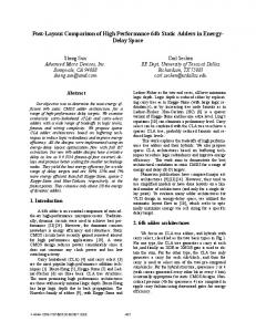
First, we focus on the expected delay per vehicle for different types of arrivals. The expected delay is computed using Little’s law ED = EL λ , where EL = ELfctl is computed by (26). In Figure 3, the expected delay is plotted as a function of the load x = cλ g for c = 60 and g = 5, 15, 30, 40. The expected delay is given in seconds instead of time-intervals, one time-interval is set to be equal to 2 seconds. Our first remark is that for arrivals with higher variability the expected delay is higher, but for each green time g the difference is really important only for a load higher than 0.8. As we can see for high load, the relative difference between expected delays for different types of arrivals is increasing with the green time. However, the absolute difference is decreasing. For load at x = 0.98(3) (the highest load in the figures) the absolute difference is given in Table 2. In the table we use EDbern , EDbinom , EDpois , EDnegbin for the expected delay in case of Bernoulli, binomial, Poisson and negative binomial arrivals respectively. From the table we see that the absolute difference is decreasing with the green time. In many approximations, see [6] and [8], the dependence on the variance is set to be linear for the fixed arrival rate, green and cycle times. However, we see that this difference increases for higher variance. Next we consider the probabilities for queue to be empty qk for k = 0, . . . , g− 1. In Figure 4, for g = 10, c = 20 and λ = 0.2, 0.3, 0.4, 0.45 these probabilities are plotted as functions of k. For the fixed g, c and λ the sum of probabilities is the same for different type of arrivals, but the distribution of this sum is different. As we see for all rates of arrivals, in the beginning of the green time the probability for queue to be empty is lower for the arrival processes that have lower variability and in the end of green time the situation is reverse. For small arrival rate, the graphs are concave, but for high load the graphs are convex. Also for low load the difference between graphs for different arrival types is smaller than for higher load.

Comparing the FCTL and one-vehicle assumptions ′ Let us first consider Xdif (1), i.e., the expected difference in the queue length between FCTL and one-vehicle models. We plot it as a function of arrival rate λ = Y ′ (1) in Figure 5. Note that if on an intersection there are at least two conflicting “main” phases, then both of them has less than half of the cycle time. Thus, in case of stable system, the arrival rate is not bigger than 0.5. If we consider, for example, 1 λ2 6 2(1−λ) 6 1 time-interval, Poisson arrivals, the expected extra delay is 2(1−λ) i.e., not more than 2 seconds. Therefore, for most of the cases the extra delay will be very small.

22

600

400

Bernoulli Binomial with n =2 Poisson Negative Binomial with n =2

200

Delay in seconds

Delay in seconds

250

Bernoulli Binomial with n =2 Poisson Negative Binomial with n =2

500

300 200

150 100 50

100 0 0.0

0.2

0.4

0.6

Load

0.8

0 0.0

1.0

0.2

0.4

a) 120

1.0

Bernoulli Binomial with n =2 Poisson Negative Binomial with n =2

80 70

Delay in seconds

Delay in seconds

80

0.8

b) 90

Bernoulli Binomial with n =2 Poisson Negative Binomial with n =2

100

0.6

Load

60 40

60 50 40 30 20

20

10

0 0.0

0.2

0.4

0.6

Load

0.8

0 0.0

1.0

0.2

0.4

c)

0.6

Load

0.8

1.0

d)

Figure 3: The expected delay as a function of load for Bernoulli, binomial, Poisson and negative binomial arrivals with c = 60, n = 2. For: a) g = 5 b) g = 15 c) g = 30 d) g = 40.

1.0

Probability to have empty queue

Probability to have empty queue

1.0 0.8 0.6 0.4

Bernoulli Binomial Poisson Negative binomial

0.2 0.0 0

1

2

3

4

5

6

Green time-interval

7

8

0.8 0.6 0.4

0.0 0

9

Bernoulli Binomial Poisson Negative binomial

0.2

1

2

3

a)

Bernoulli Binomial Poisson Negative binomial

0.8 0.6 0.4 0.2 0.0 0

1

2

3

4

5

6

7

8

9

b) 1.0

Probability to have empty queue

Probability to have empty queue

1.0

4

Green time-interval

5

6

Green time-interval

7

8

9

Bernoulli Binomial Poisson Negative binomial

0.8 0.6 0.4 0.2 0.0 0

1

c)

2

3

4

5

6

Green time-interval

7

8

9

d)

Figure 4: The probabilities qk for queue to be empty, k = 0, . . . , g−1, for g = 10, c = 20, n = 2. For: a) λ = 0.2, b) λ = 0.3, c) λ = 0.4, d) λ = 0.45.

23

60

Extra delay (in seconds)

50

Bernoulli Binomial with n =2 Poisson Negative Binomial with n =2

40

30

20

10

0 0.0

0.2

0.4

0.6

0.8

The arrival rate λ (in vehicles per time-interval)

1.0

Figure 5: The expected extra delay due to the one-vehicle assumption as compared to the FCTL assumption. Next we consider the distribution of Xdif (z), i.e., the distribution of the queue length in a bottleneck. It is plotted in Figure 6 for rate λ = 0.3, 0.5, 0.7, 0.9 vehicles per time-interval. As we see, the queue with higher variance of the arrival process has a thicker tail than the queue with lower variance. The difference between distributions increases with the arrival rate. As we derived, the absolute difference between FCTL and one-vehicle models is quite small. However, it is also interesting to know the relative difference. For the same settings as in Figure 3 we plot the relative difference of the expected queue length in Figure 7. For smaller green time the delay of FCTL model ′ is already very high and the expected difference Xdif (1) is small. Thus, the relative difference is very small. For larger green time the delay is smaller and the arrival rate is bigger, so the relative difference is bigger. As we see for g = 40, this relative difference reaches 10% for negative binomial arrivals with n = 2.

Disruption of the traffic In this subsection, we consider two types of a traffic disruption. The first one is the pedestrian/cyclist disruption and the second one is the ship/train disruption. Suppose that cyclists need 5 time-intervals, i.e., 10 seconds, to cross the road. There are two ways to provide the required green time. We can either shorten the green time of one lane, or, alternatively, extend the total cycle time and, hence, add extra red time to all lanes. Let p be the probability of cyclists arrival during the cycle. In Figure 8, we plot the overflow queue as a function of the rate for different p and g and fixed c = 60. Each graph we plot only up to load x = 0.975. The arrival process is assumed to be Poisson. As we see, the first way to deal with cyclists is highly disadvantageous for the lane. It significantly decreases the capacity of the lane and increases the overflow queue. The effect 24

1.0

Binomial with n =2 Poisson Negative binomial with n =2

0.8

0.6

Probability

Probability

1.0

Binomial with n =2 Poisson Negative binomial with n =2

0.8

0.4

0.6 0.4

0.2

0.2

0.0 0

0.0 0

1

2

3

4

5

Queue length

6

7

8

9

1

2

3

4

a) 1.0

Probability

Probability

7

8

9

Binomial with n =2 Poisson Negative binomial with n =2

0.8

0.6 0.4 0.2 0.0 0

6

b) 1.0

Binomial with n =2 Poisson Negative binomial with n =2

0.8

5

Queue length

0.6 0.4 0.2

1

2

3

4

5

Queue length

6

7

8

0.0 0

9

1

2

3

4

5

Queue length

c)

6

7

8

9

d)

0.15

Binomial with n =2 Poisson Negative Binomial with n =2

0.10

0.05

0.00 0.0

Binomial with n =2 Poisson Negative Binomial with n =2

1.0

Relative difference

Relative difference

Figure 6: Distribution of Xdif (z) for a) λ = 0.3, b) λ = 0.5, c) λ = 0.7 and d) λ = 0.9.

0.8 0.6 0.4 0.2

0.2

0.4

Load

0.6

0.8

1.0

0.0 0.0

0.2

0.4

a)

Binomial with n =2 Poisson Negative Binomial with n =2

0.8

1.0

Binomial with n =2 Poisson Negative Binomial with n =2

12

3 2 1 0 0.0

0.6

b) 14

Relative difference

Relative difference

4

Load

10 8 6 4 2

0.2

0.4

Load

0.6

0.8

1.0

0 0.0

c)

0.2

0.4

Load

0.6

0.8

1.0

d)

Figure 7: The relative difference (in %) of the expected delay in the FCTL and one-vehicle models as a function of load for binomial, Poisson and negative binomial arrivals for c = 60, n = 2 and a) g = 5 b) g = 15 c) g = 30 d) g = 40.

25

is stronger for smaller green time. The conclusion is that it is better, if possible, to increase the cycle time. As we also see from the Figure, the system with uncertainty, i.e., 0 < p < 1, has a larger overflow queue than the system without uncertainty for the same load. Consider two systems: one has no uncertainty, and another has uncertainty. Suppose that both the average green time and average cycle time are the same for these systems. Then the second system will have a bigger overflow queue, as shown in Figure 9. Let us now consider the interruption by trains/ships. We assume that with probability p all green time during the cycle is effectively red. If the probability is p = 0.0(3), c = 60, then on average there is one lost green time during an hour. In Figure 10, we plot the overflow queue as a function of the arrival rate. We see that the impact on busy lanes (with bigger green time) is larger than for lanes with short green time. Also even for small rate on both lanes the overflow queue is non-zero, as it is in the case of cyclists interruption.

Uncertain departure times Consider the FCTL model with uncertain departure times that was presented in subsection 5.2. In Figure 11, we plot the expected overflow queue as a function of the arrival rate for different probability of departure. We suppose that, on average, a vehicle departs in 2 seconds. The length of the time-interval is set to be equal to τ = 2p seconds. The arrival process is assumed to be Poisson. We fixed the cycle time (in seconds) and consider two different green times. The uncertainty in departure times does not influence the capacity of the system but only increases the the overflow queue and, consequently, the delay. The increase in the overflow queue seems to be the same. In fact, it is a bit bigger (about 0.1 difference) for the lane with smaller green time. However, this lane has a bigger overflow queue, and the relative difference for it is smaller.

Green time allocation problem In this subsection, we consider the green time allocation problem. In [11], Webster proposed to provide each lane with a part of the total green time proportional to the arrival rate, i.e., such that the load is the same for each lane. On the one hand, as we see in Figure 3, the lane with the smallest green time, i.e., with the smallest arrival rate, in this case faces the greatest delay. On the other hand, this delay is experienced by a small part of the vehicles. Let us consider an example. Suppose we have three lanes with rates’ ratio λ1 : λ2 : λ3 = 5 : 15 : 30 = 1 : 3 : 6. Suppose also that we assign to them, in total, 50 green time-intervals out of 60 time-intervals in a cycle. We consider the following ways to assign green time: • green time is proportional to the arrival rate, • green time is allocated by minimizing the expected total queue length, • green time is allocated by minimizing the maximum expected delay per lane. Due to the computational efficiency of our method we minimize queue length or delay by using a simple exhaustive search. 26

30

p=0.00 p=0.20 p=0.40 p=0.60 p=0.80 p=1.00

25 20 15

Overflow queue (vehicles)

Overflow queue (vehicles)

30

10 5 0 0.00

0.05

0.10

0.15

0.20

Arrival rate (vehicles per time-interval)

p=0.00 p=0.20 p=0.40 p=0.60 p=0.80 p=1.00

25 20 15 10 5 0 0.00

0.25

0.05

0.10

a)

p=0.00 p=0.20 p=0.40 p=0.60 p=0.80 p=1.00

25 20 15 10 5 0 0.0

0.1

0.2

0.20

0.25

0.3

0.4

0.5

b) 30

Overflow queue (vehicles)

Overflow queue (vehicles)

30

0.15

Arrival rate (vehicles per time-interval)

0.3

0.4

Arrival rate (vehicles per time-interval)

p=0.00 p=0.20 p=0.40 p=0.60 p=0.80 p=1.00

25 20 15 10 5 0 0.0

0.5

0.1

0.2

Arrival rate (vehicles per time-interval)

c)

d)

Figure 8: The overflow queue in case of cyclists as function of arrival rate. The cycle time is c = 60. The green time in figures a) and b) is g = 15 and on c) and d) g = 30. In figures a) and c) the green time for cyclists (5 time-intervals) is given from the green time of the lane. In figures b) and d) the extra time is added to the cycle.

Overflow queue (vehicles)

30 25 20 15 10

g = 14 g = 13 g = 12 g = 11 E(g) = 14 E(g) = 13 E(g) = 12 E(g) = 11

5 0 0.00

0.05

0.10

0.15

0.20

Arrival rate (vehicles per time-interval)

0.25

Figure 9: First four graphs represent overflow queue with fixed green time g = 14, 13, 12, 11. Last four graphs represent the overflow queue in case of cyclists. The cycle time is c = 60, g = 15. With probabilities p = 0.2, 0.4, 0.6, 0.8 the cyclists arrive and the green time is smaller by 5 time-intervals. The corresponding expected green time is E(g) = 14, 13, 12, 11.

27

25 20 15

30

0 train(s) per hour 1 train(s) per hour 2 train(s) per hour 3 train(s) per hour 4 train(s) per hour

Overflow queue (vehicles)

Overflow queue (vehicles)

30

10 5 0 0.00 0.01 0.02 0.03 0.04 0.05 0.06 0.07 0.08

25 20 15 10 5 0 0.0

Arrival rate (vehicles per time-interval)

0 train(s) per hour 1 train(s) per hour 2 train(s) per hour 3 train(s) per hour 4 train(s) per hour

0.1

0.2

0.3

0.4

Arrival rate (vehicles per time-interval)

a)

0.5

b)

Figure 10: The overflow queue for FCTL model with train disruption. The cycle time c = 60, the green times are a) g = 5 and b) g = 30.

Overflow queue (vehicles)

35 30

40

τ = 2.000, P (of departure) = 1.000 τ = 1.800, P (of departure) = 0.900 τ = 1.600, P (of departure) = 0.800

35

Overflow queue (vehicles)

40

25 20 15 10 5 0 0.0

0.2

0.4

Load

0.6

0.8

30 25 20 15 10 5 0 0.0

1.0

a)

τ = 2.000, P (of departure) = 1.000 τ = 1.800, P (of departure) = 0.900 τ = 1.600, P (of departure) = 0.800

0.2

0.4

Load

0.6

0.8

1.0

b)

Figure 11: The overflow queue for FCTL model with uncertain departure times. The cycle time is 120 seconds, the green times are a) 10 and b) 60 seconds. Let the total load be equal to x = 0.9. The results for Bernoulli and Poisson cases are given in Table 3. In the table, the total delay is a sum of average delays per lane. Even though it has no physical meaning, it measures the change in the expected delays. Note that for both types of arrivals all three ways of the green time allocation give similar results. However, the difference in the delay between different ways is significant, especially for the first lane. So, as we see, the proportional green time is the most beneficial for the busiest lane but very unfair for the lane with the smallest rate. Using either minimal total delay or minimal delay per lane policy improves significantly (2 times) the situation for the lane with the smallest rate but increases the delay for the busiest lane. For smaller load these three ways of the green time allocation work completely different. For the same settings c = 60, total red time equal to 10 and arrivals’ rates proportional as 5 : 15 : 30, we consider our three ways of allocation for different total loads. The result can be found in the figures 12 and 13. In the first one, the delay per lane in each type of allocation is plotted as a function of load. The second shows the allocated green time. The arrival process is assumed to be Poisson. As we see, the minimum delay per lane policy suggests almost equal green time allocation for low total load, while the minimum total queue length policy suggests to give the largest part (more than proportional 30 time-intervals) of 28

Table 3: The comparison of the expected delay and queue length for different green time allocation policies. The delay is given in seconds and the green time in time-intervals. A time-interval is set to be equal to 2 seconds.

Arrival rate λ

Lane 1 0.075

Green time Delay Queue length

5 139.626 5.236

Green time Delay Queue length

6 68.881 2.583

Green time Delay Queue length

7 56.267 2.110

90 80 70 60

Bernoulli arrivals Poisson Lane 2 Lane 3 Total Lane 1 Lane 2 0.225 0.450 0.750 0.075 0.225 Proportional green time 15 30 5 15 61.731 31.752 233.109 147.906 68.992 6.945 7.144 19.325 5.546 7.762 Minimal total queue length 15 29 6 15 61.731 38.096 168.708 71.097 68.992 6.945 8.572 18.099 2.666 7.762 Minimal delay per lane 15 28 6 15 61.731 55.355 173.354 71.097 68.992 6.945 12.455 21.510 2.666 7.762

90

Proportional policy Min total queue length policy Min delay per lane policy

80 70 60

30

30 20

10

60

0.4

0.6

Total load

0.8

00.0

1.0

29 48.670 10.951

188.759 21.378

0.2

0.4

0.6

Total load

0.8

1.0

b)

80

Proportional policy Min total queue length policy Min delay per lane policy

70 60

Proportional policy Min total queue length policy Min delay per lane policy

50

Delay

50

40

40

30

30

20

20

10

10 00.0

188.759 21.378

10 0.2

Total queue length

70

29 48.670 10.951

Proportional policy Min total queue length policy Min delay per lane policy

a)

80

254.807 21.838

40

20

90

30 37.909 8.529

Delay

40

00.0

Total 0.750

50

Delay

50

arrivals Lane 3 0.450

0.2

0.4

0.6

Total load

0.8

00.0

1.0

c)

0.2

0.4

0.6

Total load

0.8

1.0

d)

Figure 12: The delay per lane and the total queue length as function of total load for different ways of green time allocation. Figures a), b) and c) represent delay on lanes with low, medium and high arrivals’ rates. Figure d) is the graph of the total queue length.

29

green time to the third lane with the highest arrival rate. The difference in delay for different policies is clearer for the lowest and highest arrival rate lanes. We also see that the total queue length for proportional policy and minimum total length are almost the same. However, we already saw from the table how significant the difference in the delay is (especially for the first lane). For lanes 1 and 2 (low and medium rate) the minimum delay per lane policy is the most beneficial, while for the third lane it is the most disadvantageous. The minimum total length policy is conversely the most beneficial for the busiest lane and the most disadvantageous for the first two lanes. However, for higher load it gives smaller delay than the proportional policy.

Conclusions We presented in this paper a new method to calculate the expectation and distribution of the queue length for a number of discrete-time queueing systems. We applied this method to the FCTL model and several of its extensions. First, we studied the impact of arrival variability. The numerical results show that higher variance of the arrival process results in higher average delay, but the difference is noticeable only for a load higher than 0.8. We compared the FCTL and one-vehicle assumptions. The absolute difference is quite small for many relevant applications, however the relative difference can be quite big. Additionally, we proved the decomposition rule for the onevehicle model. Comparing different disruptions of the traffic we found several interesting results. For example, the green time for cyclists or pedestrians is better to add to the cycle length than to give from the green time of one of the lines. Also the disruptions caused by trains and ships have a serious impact on the expected overflow queue and, consequently, the average delay. This kind of disruption causes the increase in the overflow queue even for a low load, while the disruption by cyclists and the uncertainty in departure time result in a overflow queue that is close to zero for low load. The uncertainty in departure times has the smallest impact on the overflow queue among considered types of disruption. It does not influence the stability of the system and the change in the overflow queue is relatively small. Finally, we compared different green time allocation policies and concluded that the proportional policy may be extremely disadvantageous for the lanes with small arrival rate. The minimal total queue length policy may give too much priority to the busiest lanes, while the minimal delay per lane policy favours the lanes with lowest arrival lane. The choice of policy heavily depends on the goals of control. The future work will be on extending this method to a wider range of models. For example, for the actuated control of an intersection.

Appendix. The proof of Theorem 1 ¯ 1 . ConRecall that we need to P prove that zB(w) 6= wB(z) for z 6= w, z, w ∈PD ∞ ∞ ˜ sider Taylor expansion j=0 bj z j of B(z) around zero. Let B(z) = j=2 bj z j . ˜ ˜ Then, it is equivalent to prove that z(b0 + B(w)) 6= w(b0 + B(z)) for z 6= w, 30

¯ 1 . Now, we can reformulate the theorem in the following way: there is z, w ∈ D ˜ ¯ 1 for each a ∈ C. not more than one root of the equation z = a(b0 + B(z)) in D ¯ 1 . To make such a Number a here represents the value b +w for some w ∈ D ˜ 0 B(w) ˜ ¯ 1. reformulation we need to show that b0 + B(w) 6= 0 for all w ∈ D ˜ First we show it for w = 1. Consider the derivative of B(z) at 1. On one ˜ ′ (1) = B ′ (1) − b1 < hand, according to the stability assumption, we get that B ˜ 1 − b1 = B(1) + b0 . On the other hand, bk > 0 for k ∈ N, and, thus, ˜ ′ (1) = B

∞ X

jbj >

j=2

∞ X

˜ 2bj = 2B(1).

j=2

˜ ˜ ′ (1) < B(1) ˜ ˜ Finally, we get that 2B(1) 6B + b0 . Therefore, b0 > B(1). Now, we need to use the following small lemma: P∞ Lemma 4. Consider an analytic function C(z) = j=0 cj z j in Dr+δ , where r ∈ R, δ > 0. Suppose that cj > 0 for all j ∈ N ∪ {0}, then the absolute value ¯ r. of C(z) reaches the maximum value in r, i.e., |C(z)| 6 C(r) for each z ∈ D Proof. Since the function C(z) is in disk Panalytic P∞Dr+δ , Taylor series converges ∞ absolutely. Therefore, |C(z)| 6 j=0 cj |z|j 6 j=0 cj rj = C(r).

˜ ¯ 1 , and, consequently, As a corollary we get that |B(z)| < b0 for each z ∈ D ˜ ¯ there are no solutions of the equation b0 + B(z) = 0 in D1 . Hence, it is sufficient to prove that equations ˜ z = a(b0 + B(z)) (35)

¯ 1 for each a ∈ C. has not more than one root in D If a = 0, we have the simple equation z = 0 that has not more than one solution. If a 6= 0, we can uniquely represent it as teiϕ , where 0 6 ϕ < 2π, t > 0. We want to prove, for a fixed value of ϕ, that the amount of roots inside the unit disk does not increase when t increases. To do so, we consider our roots as functions of t and prove that the absolute value of the root increases as t increases. Suppose z(t) is a root of the equation (35) inside the unit disk. Consider its derivative: dz d ˜ ˜ ˜ ′ (z) dz . = (teiϕ (b0 + B(z))) = eiϕ (b0 + B(z)) + teiϕ B dt dt dt Rearranging and plugging

z ˜ t(b0 +B(z))

t

instead of eiϕ give us

dz z . = ˜ ′ (z) z B dt 1− b + ˜ B(z) 0

Thus, the derivative of the |z(t)|2 is equal to   d(z z¯) dz dz d¯ z 2|z|2 .  = z¯ + z = 2Re z¯ = ˜ ′ (z) B dt dt dt dt tRe 1 − bz+ ˜ B(z) 0

To prove that this derivative is positive we only need to prove the following lemma.

31

Lemma 5. There is some δ > 0 such that for each z ∈ D1+δ ! ˜ ′ (z) zB > 0. Re 1 − ˜ b0 + B(z)

(36)

¯ 1. Proof. First of all, it is sufficient to prove that (36) holds for each z ∈ D Indeed, if for some point z inequality (36) holds, then for some neighbourhood ¯ 1 is compact, if (36) holds in D ¯ 1 , it also holds for of z it also holds. Since D small neighbourhood D1+δ , δ > 0. Now note that inequality (36) is equivalent to the following inequality:   ˜ ˜ z )) − z B ˜ ′ (z)(b0 + B(¯ ˜ z )) > 0. Re (b0 + B(z))(b 0 + B(¯

  ˜ ′ (z) − B(z) ˜ ˜ z )) + (z B ˜ ′ (z) − B(z)) ˜ ˜ z) . It can be rewritten as b20 > Re b0 (z B − B(¯ B(¯ ˜ z )) = Re(B(z)), ˜ Since Re(B(¯ we finally get that (36) is equivalent to   ˜ ′ (z) − 2B(z)) ˜ ˜ ′ (z) − B(z)) ˜ ˜ z) . b20 > Re b0 (z B + (z B B(¯ (37)

Note that Re(z) 6 |z| for each z ∈ C, and, thus,   ˜ ′ (z) − 2B(z)) ˜ ˜ ′ (z) − B(z)) ˜ ˜ z ) 6 b0 |z B ˜ ′ (z)−2B(z)|+|z ˜ ˜ ′ (z)−B(z)|·| ˜ ˜ Re b0 (z B + (z B B(¯ B B(z)|. ˜ ′ (z) − 2B(z), ˜ ˜ ′ (z) − B(z) ˜ ˜ Since functions z B zB and B(z) are analytical and have positive coefficients in their Taylor expansion at 0, we can use lemma 4. This gives us that   ˜ ′ (z) − 2B(z)) ˜ ˜ ′ (z) − B(z)) ˜ ˜ z) 6 Re b0 (z B + (z B B(¯ ˜ ′ (1) − 2B(1)) ˜ ˜ ′ (1) − B(1)) ˜ ˜ ˜ ˜ 6 b0 ( B + (B · (B(1)) < b0 (b0 − B(1)) + b0 B(1) = b20 .

˜ ′ (1) < B(1)+b ˜ ¯ Here we used that B 0 . Thus, we proved for each z ∈ D1 inequality (37), which is equivalent to (36). z¯| ˜ We proved that d|z dt > 0 for each z = z(t) ∈ D1+δ \{0}. Since b0 + B(0) 6= 0, we get that z(t) 6= 0. Therefore, any root of the equation (35) for t > 0 goes ¯ 1+δ . Hence, the amount of roots inside D1 decreases when t increases. outside D But for small t > 0 we can use Rouche’s theorem to show that there is only one root of the equation (35). Thus, we have proved Theorem 1.

References [1] I. J. Adan, J. van Leeuwaarden, and E. M. Winands. On the application of rouch´e’s theorem in queueing theory. Operations Research Letters, 34(3):355–360, 2006. [2] N. T. Bailey. On queueing processes with bulk service. Journal of the Royal Statistical Society. Series B (Methodological), pages 80–87, 1954. [3] J. Darroch. On the traffic-light queue. The Annals of Mathematical Statistics, 35(1):380–388, 1964. 32

[4] A. J. Janssen and J. S. van Leeuwaarden. Analytic computation schemes for the discrete-time bulk service queue. Queueing Systems, 50(2-3):141–163, 2005. [5] D. R. McNeil. A solution to the fixed-cycle traffic light problem for compound poisson arrivals. Journal of Applied Probability, 5(3):624–635, 1968. [6] A. J. Miller. Settings for fixed-cycle traffic signals. OR, pages 373–386, 1963. [7] G. F. Newell. Approximation methods for queues with application to the fixed-cycle traffic light. Siam Review, 7(2):223–240, 1965. [8] M. S. van den Broek, J. van Leeuwaarden, I. J. Adan, and O. J. Boxma. Bounds and approximations for the fixed-cycle traffic-light queue. Transportation Science, 40(4):484–496, 2006. [9] J. S. van Leeuwaarden. Delay analysis for the fixed-cycle traffic-light queue. Transportation Science, 40(2):189–199, 2006. ˙ B. Vinberg. A course in algebra. Number 56. American Mathematical [10] E. Soc., 2003. [11] F. V. Webster. Traffic signal settings. Technical report, 1958.

33

35

Green time lenght

30

40

Lane 1 Lane 2 Lane 3

35 30

Green time lenght

40

25

Lane 1 Lane 2 Lane 3

25

20

20

15

10

15

10

5

5

00.0

00.0

0.2

0.4

0.6

Total load

0.8

1.0

a)

0.2

0.4

0.6

Total load

0.8

1.0

b)

Figure 13: The green time allocated to each lane for a) minimum delay per lane policy and b) minimum total queue length. Lanes 1, 2, 3 correspond to the lanes with low, medium and high arrival rate.

34