Exact Radon Rebinning Algorithm for the Long. Object Problem in Helical Cone-Beam CT. S. Schaller*, Associate Member, IEEE, F. Noo, Associate Member, ...
IEEE TRANSACTIONS ON MEDICAL IMAGING, VOL. 19, NO. 5, MAY 2000
361
Exact Radon Rebinning Algorithm for the Long Object Problem in Helical Cone-Beam CT S. Schaller*, Associate Member, IEEE, F. Noo, Associate Member, IEEE, F. Sauer, K. C. Tam, G. Lauritsch, and T. Flohr
Abstract—This paper addresses the long object problem in helical cone-beam computed tomography. We present the PHI-method, a new algorithm for the exact reconstruction of a region-of-interest (ROI) of a long object from axially truncated data extending only slightly beyond the ROI. The PHI-method is an extension of the Radon-method, published by Kudo, Noo, and Defrise in issue 43 of journal Physics in Medicine and Biology. The key novelty of the PHI-method is the introduction of a virtual for each value of the azimuthal angle in the object image space, with each virtual object having the property of being equal to the true object in some ROI . We show that, for each , one can calculate exact Radon data corresponding to the two–dimensional (2-D) parallel-beam projection of onto the meridian plane of angle . Given an angular range of length of such parallel-beam projections, the ROI can be exactly reconstructed because is identical to in . Simulation results are given for both the Radon-method and the PHI-method indicating that 1) for the case of short objects, the Radon- and PHI-methods produce comparable image quality, 2) for the case of long objects, the PHI-method delivers the same image quality as in the short object case, while the Radon-method fails, and 3) the image quality produced by the PHI-method is similar for a large range of pitch values.
()
()
()
()
()
Index Terms—Cone-beam CT, image reconstruction, long object problem, radon method.
I. INTRODUCTION
T
HIS paper is about exact three-dimensional (3-D) image reconstruction in helical cone-beam (CB) computed tomography (CT). We propose here a solution to the long-object problem, which consists in achieving exact reconstruction of a finite region-of-interest (ROI) in a long object from helical data which extend only slightly beyond the ROI. Until now, no solutions were known for this problem. Helical cone-beam CT means that CB data acquisition is considered with a helical motion of the source-detector assembly relative to the patient. Using a helical path for data acquisition
Manuscript received September 1, 1999; revised February 14, 2000. This work was supported by the Bayerische Forschungsstiftung. F. Noo is a chargé de recherches with the Belgian National Fund for Scientific Research (F.N.R.S., Belgium). The Associate Editor responsible for coordinating the review of this paper and recommending its publication was M. Defrise. Asterisk indicates corresponding author. *S. Schaller, G. Lauritsch, and T. Flohr are with Siemens Medizinische Technik, Forchheim, Germany. F. Noo is with the Institute d’Electricité Montefiore, Université de Liège, B-400 Liège, Belgium. F. Sauer and K. C. Tam are with the Siemens Corporate Research, Inc., Princeton, NJ 08540 USA. Publisher Item Identifier S 0278-0062(00)05269-1.
has been recommended in medical imaging since the appearance of spiral CT in the late 1980’s [1]–[3]. The helical path permits a fast 3-D data acquisition by combining a smooth translation of the patient with a uniform rotation of the source-detector assembly. Fast data acquisition is important for increasing patient throughput in screening studies, reducing motion and respiratory artefacts and making good use of the available sustained X-ray power. With a helical path, the speed of data acquisition is determined by the value of the helix pitch. The higher the pitch, the faster the data acquisition. But using large pitch values requires suitable equipment: large area detectors and CB collimation of the X-ray source are needed to collect sufficient data for image reconstruction. The fabrication of high-quality area detectors and the design of appropriate reconstruction algorithms are the two main challenges in the development of a helical CB CT scanner. Recent progress in detector technology has inspired a number of researchers to work on reconstruction algorithms. Before manufacturing a helical CB CT scanner, basic questions, like, e.g., “is it worth building hardware for CB backprojection?” must be answered. To answer such questions, development of several different reconstruction algorithms is needed, while keeping in mind that careful algorithm comparison will be necessary at some point. For efficiency purposes, analytic reconstruction algorithms are preferred to iterative methods. In the class of analytic reconstruction algorithms, distinction is made between exact methods and approximate methods. Approximate algorithms generally have the virtue of being computationally less expensive than exact methods. However, due to their intrinsic approximations, they introduce artefacts which generally increase with increasing cone angles. Several medical CT manufacturers have recently introduced multirow CT systems with a small number of detector rows, i.e., very small cone angles. For these small cone angles, it has been shown that 2-D filtered backprojection methods combined with axial interpolation provide sufficient image quality [4], [5]. For the axial interpolation, different approaches have been proposed in [6]–[8]. For intermediate cone angles, approximate methods employing true 3-D backprojection are to be preferred to the above 2-D methods. The first approximate algorithms of that class were direct adaptations of the well-known Feldkamp algorithm [9] to the helical path (see, e.g., [10]–[12]). These direct adaptations have some weaknesses. The detector is not efficiently utilized, which induces artificial limitations on the pitch value,
0278–0062/00$10.00 © 2000 IEEE
362
IEEE TRANSACTIONS ON MEDICAL IMAGING, VOL. 19, NO. 5, MAY 2000
and thereby on the speed of data acquisition. Furthermore, the X-ray dose applied to the object is not fully exploited, which is inappropriate for medical imaging purposes. Recent advances overcoming these problems have been reported in [12], [14] where CB Backprojection is only performed on a short-scan helix segment, and in [15] where data are rebinned to an intermediate parallel data set. Yet another approach, reported in [16] attempts to benefit from the 3-D backprojection while avoiding its additional costs by using Fourier techniques. In contrast to approximate algorithms, exact methods avoid intrinsic approximations and can therefore provide superior image quality for large cone angles. The main difficulty to overcome in the development of these algorithms is axial data truncation, which cannot be avoided in medical imaging, as obtaining axially untruncated data would require having a detector that covers the patient from head to toe. If the data were not truncated, several CB algorithms proposed in the literature would be appropriate for reconstruction. With truncation, things are more complicated and it is only recently that solutions have been proposed in [20], [21]. As in [17]–[19], reconstruction in [20], [21] is based on the calculation of Radon data (plane integrals) from which the 3-D image volume is obtained by Radon inversion. The keypoint is in the calculation of the Radon data which is performed by data combination: in [20], [21], plane integrals are calculated by assembling triangular patches obtained from different projections. The methods of [20], [21] are not very attractive for practical applications because they assume that the helical path cover the whole length of the object, even though the ROI is a small axial region of the object. Technically speaking, we say that the methods of [20], [21] are not suitable for the long object problem. A modification to [20], [21] to solve the long object problem was proposed by Tam in [22]. Unfortunately, this solution requires the addition of two circles to the helical vertex path, which make the data acquisition impractical in some cases. This paper presents a new method that solves the long object problem using only the helical path. This method, called the PHI-method [23], [24], [26], is also based on the results of [20], [21]. The organization of the paper is as follows. In Section II, we introduce first the scanner setup with our notation. Next, in Section III, we review the Radon-method reported in [21] for entire object reconstruction from truncated projections. The PHI-method can be seen as an extension of the Radon-method. Section IV provides all necessary details to understand how the PHI-method works. Section V is then dedicated to experiments. We show results obtained from computer simulations to illustrate the performances of the PHI-method. Conclusions are given in Section VI. II. SCANNER GEOMETRY AND NOTATIONS Let , , and denote Cartesian coordinates in and let be the density function describing the object under study, . In this work, we consider that is smooth with and may be nonzero everywhere inside the cylindrical region
(1)
Fig. 1. Helical cone-beam data acquisition. The region-of-interest is that part of the long cylinder between z and z . The helix extends slightly and � . beyond the ROI. Its limits are given by �
However, only the finite region (2) inside that region-of-interest is of interest. To reconstruct (ROI), we collect cone-beam (CB) projections along the helical vertex path (3) In this expression, and represent the radius and the pitch . Limits and of the helix, respectively, with are finite numbers which define the axial extent of the helix. For , we consider that the helix should reconstruction of the ROI , which implies only slightly extend beyond the limits of and (see Fig. 1). The area detector is planar and moves with the cone vertex, so that the detector plane is always parallel to the -axis and to tangent to the path. To describe the the vector CB geometry, we introduce three unit orthogonal vectors
and (4) is orthogonal to the detector plane, while and Vector define the orientation of detector pixels in the -system. The location of a detector pixel in the detector plane is specified using two Cartesian coordinates, and . These coordinates are is at the orthogonal projection defined such that onto the detector plane. Fig. 2 depicts the situation. of The CB projection obtained at position is the set of line to the detector pixels. This projection integrals connecting is denoted
(5)
SCHALLER et al.: EXACT RADON REBINNING ALGORITHM FOR THE LONG OBJECT PROBLEM
Fig. 2. Cone-beam geometry. Vectors e , e , and e are orthogonal; e is orthogonal to the detector plane, e is parallel to the z -axis. A point in the detector plane is located using Cartesian coordinates (u; v).
Fig. 3. Definition of region B . The curves V (u) and V (u) bounding B are the projections of the helix turns that are just above and below the vertex point a(�).
In this equation, represents the part of the detector plane -domain] where data are measured, while is the dis[ tance from the cone vertex to the detector plane. Data truncation is allowed in the -direction. In other words, for a given , the -extent of does not need to include all lines where is nonzero. Note that is independent of because we assume the area detector moves with the cone vertex. In [21], [22], [25], it is shown that exact reconstruction is posbe the region sible when the following condition is met. Let is nonzero. The area deof the detector plane where tector must be sufficiently large, so that for each , where is the set of -pixels located between the curves (6) and
363
Fig. 4. Location of 5(�; '; l) in the (x; y; z )-space.
first step, the CB data are used to calculate samples of the deriva. In the second step, tive of the 3-D Radon transform of is obtained from the Radon data evaluated in the first step, using a Radon-inversion formula. In Section III-A, we give some details on the Radon transform. Next, in Section III-B, we describe the Grangeat formula [21] which permits to convert CB data into Radon data when CB data are not truncated. Section III-B helps understanding Section III-C where a modified Grangeat formula [21] is introduced. This modified formula is the key point in the Radonmethod. As explained in Section III-D, it can be used in a data combination process to calculate Radon data from truncated heis met (see lical CB data, provided the condition end of Section II). By concept, the Radon-method only applies to short-object geometries. In Section III-E, we discuss problems which occur when trying to apply the Radon-method to a long object geometry. This discussion leads to the notion of missing data and contaminated data which are useful to understand how the long object problem is solved in the PHI-method of Section IV. A. Radon Transform is a By definition the Radon transform of the function the integral new function which associates to each plane of onto this plane. Let be the plane that is at the of signed distance from origin and orthogonal to the vector (8) as shown in Fig. 4. We write the Radon transform of function of and of the spherical angles and
as a
(9) (7)
In this work, we will assume that this condition holds. Geometand represent the CB projection of the rically, , using as cone vertex (see helix turns above and below and Fig. 3). Due to the rotational invariance of the helix, are independent of .
Mathematical properties of the Radon transform can be easily accessed in the literature (see, e.g., [27]). Here, we will only recan be reconstructed from provided call that is known for all planes passing through a neighborhood of point . In CB tomography, one has no direct access to but its derivative with respect to
III. RADON-METHOD In this section, we review the Radon-method published in [21]. This reconstruction method proceeds in two steps. In the
(10)
364
IEEE TRANSACTIONS ON MEDICAL IMAGING, VOL. 19, NO. 5, MAY 2000
where the dot denotes the scalar product and is the gradient, can be calculated. For this modified can be reconstructed transform, the same property holds: provided is known for all planes from passing through a neighborhood of point . from Several algorithms can be designed to reconstruct (see, e.g., [28]–[30]). Fundamentally, any choice can be made. The only important point one must concentrate from its helical CB data is to on to reconstruct from . know how to obtain the values of This point is addressed through the next three sections for the Radon-method. B. Grangeat’s Formula Grangeat’s formula only applies to nontruncated projections. be such a projection and define Let (11) as the line in the detector plane that is orthogonal to vector at signed distance from the origin (see Fig. 5). We calculate (12) with
Fig. 5. Schematic representation of the Grangeat formula. Top: 3-D view of the detector and the cone vertex. Bottom: view of the detector plane. The line L(s; �) in the detector plane and the vertex a(�) defines a plane 5 on which f (�; '; l) can be calculated. The vector n is orthogonal to 5. The line L(s; �) is orthogonal to the vector � = (cos �; sin �) at signed distance s from the origin (u; v ) = (0; 0).
R
C. Modified Grangeat’s Formula (13) represents, up to a weight factor and a Physically, on . Grangeat’s derivative filter, the integral of and . formula establishes a link between This link is (14) where vector
and
are the spherical coordinates of
(15) and (16) and the Fig. 5 illustrates the situation. The line define a plane orthogonal to and cone vertex is the value of on this plane. , Grangeat’s formula yields all Given a projection on planes containing the vertex point values of . To reconstruct in region , one just needs to on all planes which intersect . This calculate task is possible using Grangeat’s formula provided data are also intersect nontruncated and all planes which intersect the vertex path. The helical trajectory satisfies this latter and are suitably chosen. condition when the limits
is truncated in . In Consider that the CB projection of (12) cannot be calculated such a case, the function , as shown in Fig. 6. Grangeat’s formula thus for all lines on all planes confails in giving access to values of . The purpose of this section is to define what can taining in the presence of axial truncation. be obtained from Two cases must be considered, depending on the location of in the detector plane. If does not cross the mea. surement region, then nothing can be obtained from crosses the measurement region, then If, on the contrary, on the plane conpartial or complete calculation of and is possible using a modified Grangeat taining formula [21]. which crosses the measurement reConsider a line and to describe the gion, as shown in Fig. 6, and use with that region. The modified intersection points of Grangeat formula can be written as follows. Let
(17) with have
defined as in Section III-A [see (13)]. Then, we
(18)
SCHALLER et al.: EXACT RADON REBINNING ALGORITHM FOR THE LONG OBJECT PROBLEM
365
\D
Fig. 7. Definition of parameters t and t using the restricted region B . Top: Example where t and t are defined by V u and V u , respectively, i.e., by the boundaries of the region B . Bottom: Example where t is defined by the boundary of and t is defined by V u , i.e., by the top boundary of B .
() ()
D
Fig. 6. Schematic representation of the modified Grangeat formula. Top: 3-D view of the detector and the cone vertex. Bottom: view of the detector plane. The line L s; � crosses the measurement region but g u; v; � has nonzero values on parts of L s; � outside that region. The modified Grangeat formula yields the part of f �; '; l that corresponds to the integration region defined by the segment t ; t and a � .
( ) ( ) R ( ) [ ] ()
(
)
1
where is given by (15) and is the triangle and the segment on the line . defined by Formula (18) is to be understood as follows: on are zero outside 1) if all values of yields the the measurement region, then on the plane defined by and value of ; is nonzero on parts of outside the 2) if measurement region, as in Fig. 6, then yields the part of that corresponds to the ; compare (18) to (10). integration region only applies As defined above, the function which cross the measurement region. When to lines does not cross the measurement region, we said that does not bring contribution to the the CB projection . This point can be incorporated into calculation of by taking for the definition of which do not cross the measurement region. We lines will adopt this extended notation in the following sections. D. Data Combination is calculated in the RadonWe now explain how intersects the helical method. Consider that the plane , with for any path at vertices . The key idea in the Radon-method is to build by data combination as follows: (19)
()
In this expression, and define the line where intersects the detector plane for projection , and is obtained from according to (17). For (19) to hold, some strong conditions must be assumed on the limits of the measurement region for each projection . corresponds to a Recall from Section III-B that . This triangle is defined by and the triangle which is within the measurement resegment of line gion for projection . To simplify the exposition, we denote it . The modified Grangeat formula states that (20) with
orthogonal to
. Equation (19) implies thus (21)
Comparing
(21) with (10), one sees that triangles , cannot be arbitrary. One must have for
(22)
and (23) where so that each point in the region of plane is nonzero belongs to one and only one triangle . Such conditions can only be met by assuming a very specific form for the . measurement region for each projection Assume that the helix extends well beyond the limits of the . Assume also that as stated at support of the end of Section II. In such a case, it is shown in [21] that (19) which intersects , provided the is valid for any plane is used to define the parameters and in the region , as illustrated in Fig. 7. Region is calculation of
366
IEEE TRANSACTIONS ON MEDICAL IMAGING, VOL. 19, NO. 5, MAY 2000
R (
)
Fig. 8. Illustration of triangles used to build f �; '; l in the Radon-method for a plane that has N intersections with the helix. Top: 3-D view of the helical source trajectory a � , the object and the integration plane . Bottom: View of the integration plane . The triangle is defined in the plane by the lines which connect a � to a � and a � .
5
=3 () 5 ( ) (
)
1
(
)
5
5
Fig. 9. Long-object problem. This figure is similar to Fig. 8 except for the object that now extends beyond the limits of the helix. Data combination formula of the Radon-method cannot be applied because data are missing to define triangles which completely cover the region where f x is nonzero in the plane .
()
5
considered as a mask delimiting the useful pixels in . Using to get , the triangles involved in (19) are limited by lines connecting consecutive vertices together in (see Fig. 8). Conditions (22) and (23) are satisfied by construction. Some warnings are warranted concerning calculation of on lines which intersect the upper or lower at two points. For these lines, the boundary of region definition of and is more complicated than what is shown in Fig. 6. We refer to [21, pp. 2893–2894] for specific details. E. The Long Object Problem In this section, we discuss the problems which occur in the Radon-method when the helical path does not extend well beyond the limits of the object. As explained below, the situation can be seen in two different ways, which leads either to the notion of missing data or to the notion of contaminated data. In both cases, the bottom line is always the same: for any point in the ROI, there exist planes containing for which cannot be exactly obtained. Since achieving exact reconstrucwith inaccurate Radon data is impossible, one must tion of conclude that the Radon-method fails to solve the long-object problem. We first examine what happens when the Radon-method is directly applied to the measured data, as described in the previous sections. The difficulties which arise in that case are easy to picture (see Fig. 9 which illustrates the decomposition into for a vertical plane ). Due to a lack of CB projectriangles tions, we observe that data combination can only be performed
Fig. 10. Data combination for a virtual object in the Radon-method. The dark-gray region correspond to . Projections � and � are missing but triangles , , and can be defined to completely cover . Here, and are given a definition different from the one adopted in Fig. 8.
1
1 1 1
1
\5
\5
to cover the central part of the object in . Triangles are is nonzero. missing to cover the whole region of where Therefore, the Radon value on cannot be exactly calculated. Unfortunately, Fig. 10 illustrates only the case of a single plane . When rotating about the -axis, one obtains the situation of Fig. 11. There are no more vertices on the top and in and triangles which exactly cover bottom lines limiting cannot be defined. Therefore, the Radon value on cannot be exactly calculated by data combination. Here, when trying to define triangles, one sees that data are either missing or
SCHALLER et al.: EXACT RADON REBINNING ALGORITHM FOR THE LONG OBJECT PROBLEM
Fig. 11. Data contamination for a virtual object in the Radon-method. f �; '; l by For this plane, no triangles can be defined to calculate data combination. The white region is called a contaminated region because f x in this region. Contaminated regions must be avoided in f x . But this is only possible by introducing the the definition of triangles black region which corresponds to missing information for calculation of f �; '; l .
( ) 6= ( )
R (
)
R (
)
1
contaminated by values of at points where . . This data contamination affects the calculation of Intuitively, when using a short helical path for a long object, . one should not expect to reconstruct more than some ROI It is therefore a good suggestion to introduce a virtual object if else
(24)
and to focus the calculations in the Radon-method on obtaining instead of . In Fig. 10, we show how things could work for a vertical plane. In this figure, the reis a rectangle and triangles can be defined to exgion actly cover this region without overlapping. Using these triangles for data combination, one can exactly obtain the desired Radon value. The only difference with respect to the original Radon-method is that a mask different from must be used for the projections corresponding to the top and bottom triangles. In the PHI-method, situations such as that of Fig. 11 are avoided to only deal with situations similar to that of Fig. 10. to To achieve this goal, we allow the virtual object be replaced by a family of virtual objects depending on the orientation of the integration planes.
Fig. 12.
Definition of the meridian plane
367
5
.
for each -value. A key point to note is that this calculation is not carried out on the same set of planes for each . For , is only calculated on planes orthogonal to the meridian plane (25) ). The planes where (see Fig. 12 for a description of is calculated are chosen so that the parallel-beam onto can be obtained in the region projection of . Since and are identical on , one on all thereby obtains the parallel-beam projections of , for points in . Mathematically, with planes can be easily reconstructed from these projections, as in the two-stage algorithm of Marr [28] for Radon inversion. This section is broken down in four parts. We begin with the definition of virtual objects in Section IV-A. Next, in Seccan be calculated on tion IV-B, we explain how . Section IV-C shows how to carry out planes orthogonal to -values to parallel-beam the transformation from , and how to reconstruct in from projections of these parallel-beam projections. The results of Sections IV-B and IV-C are summarized in Section IV-D with a description of the PHI-method in pseudocode and a discussion on specific aspects of the method, such as the scan range that is required for . reconstruction of a given ROI A. Virtual Objects
IV. PHI-METHOD In the PHI-method, efforts are focussed on the reconstruction using a helical path which only of the cylindrical ROI (see Section II for the definition of cover a bit more than and ). To reconstruct this ROI, we introduce virtual objects in . These that have the property of being identical to virtual objects are defined using the azimuthal angle in the -space: for each value of , we define a virtual to describe that object. In [26], we object and a function defined the local ROI to be the region where each function is supported. Here, the data combination idea of Section III-D is applied to calculate the derivative of the Radon transform of functions
, we use the plane and To define the virtual object lines orthogonal to that plane. Let and be Cartesian coordi, with point at origin . nates in and It is easy to show that the line which is orthogonal to hits at point such that contains the cone vertex (26) varying from to , (26) defines a sine wave in (see Fig. 13). This sine wave is the parallel-beam . Let and be the projection of the helical path onto which extends from to first and last segments of and correspond to half helix-turns. Geometrically, the
With
368
IEEE TRANSACTIONS ON MEDICAL IMAGING, VOL. 19, NO. 5, MAY 2000
Fig. 13. Illustration of curves C meridian plane 5 .
and C
on the sine wave S (�) in the
Fig. 15. One-to-one relation between planes 5(�; '; l) orthogonal to 5 and lines L(�; l) in 5 .
B. Radon Data can be calcuIn this section, we explain how which are orthogonal to and lated on the planes ; is fixed for all the discussion. Before going into intersect details, observe that there is a one-to-one relation between the orthogonal to and the lines planes (28)
Fig. 14. to 5 .
Support of the virtual object f
(x). The vector e
lines which are orthogonal to and touch and inside the cylinder . Volume a finite volume support of the virtual object at angle and we have if otherwise.
is orthogonal
define is the
(27)
Figs. 13 and 14 illustrate this definition; Fig. 13 shows curves and in , and Fig. 14 shows in the -space. Note that in Fig. 13, we assumed that the region is between the curves and . To use the PHI-method, this condition must be fulfilled for all -values. In Sections IV-B is between and . In Section and IV-C, we assume IV-D, we discuss the implications of this condition on the scan in . range required to reconstruct
(see Fig. 15). To know if intersect , we in crosses the region . Simicheck whether or not larly, to know how many vertices are in , we count the number of intersection points between and the sine wave of Fig. 13. The lines which cross the region can be listed in two classes. There are the lines which intersect or , or and , and there are the lines which have no intersecboth and . Recall that and are used to delimit tions with of , as shown in Figs. 10 and 11. When the support intersects either or , or both and , data may be missing to calculate using (19). The situation was illustrated in Fig. 9. Problems may occur because the axial extent of the helix is not required to cover the whole region where can be nonzero. The calculation of is, however, always possible, as explained below. inWe begin the discussion with the situation where and as shown in Fig. 16. To caltersects both curves culate , we use a subset of vertices which are in . We use the two vertices which are on the lines orwhere meets and , and we use the thogonal to vertices which are projected between and on . These with . We consider that vertices are denoted for any so that corresponds to the intersection of with and to the intersection of with . The vertices have some particularities. They permit to which completely cover, without overlapdefine triangles ping, the region where is nonzero in . These triangles are as follows: is limited on one side by the line connecting • to and on the other side by the line which contains and is orthogonal to , i.e., by the line where intersects ;
SCHALLER et al.: EXACT RADON REBINNING ALGORITHM FOR THE LONG OBJECT PROBLEM
369
Fig. 17. Definition of masks used to apply the modified Grangeat formula in the PHI-method. Top: Mask applied for vertex points a(�) which lie on C when projected onto 5 . Middle: Mask applied for vertex points a(�) which lie neither on C nor on C , but inbetween, when projected onto 5 . Bottom: Mask applied for vertex points a(�) which lie on C when projected onto 5 .
Fig. 16. Data combination for a line L(�; l) crossing C and C (N = 6). Top: View onto 5 . Bottom: View onto the integration plane 5(�; '; l).
• for , is limited by the two lines to and ; connecting • is limited on one side by the line connecting to and on the other side by the line which contains and is orthogonal to , i.e., by the line where intersects . Fig. 16 illustrates this definition. By construction, there is no and for and overlapping between (29) and are identical at almost every point Furthermore, of for any -value, because . Using the Lebesgue integral, we can thus write1 that
In this equation, and define the line where intersects the detector plane for projection , and is obtained from according to (17). For (31) to hold, some particular regions must be and in the calculation of used to define the parameters . These regions are constructed from region of Fig. 3 as follows: is the subset of pixels in which have a coordinate • ; • is identical to for ; is the subset of pixels in which have a coordinate • (see Fig. 17). , recall that To understand this definition for is bounded by lines connecting to other vertices, i.e, on the boundaries of . For by lines which hit the detector or , the situation is different. One side of corresponds to a line connecting to another vertex, while . The former the other corresponds to a line orthogonal to line hits the detector on a boundary of . The latter one hits , which explains the same detector at a pixel of coordinate and . the definition of because Mathematically, (31) does not deliver at the upper and lower boundaries the discontinuities of introduce differences between and of
(30) (32) . At this stage, we where is the vector orthogonal to can use the modified Grangeat formula to calculate each term on the right-hand side (RHS) of (30), which leads to
We show in the Appendix that the following equation must be : used to obtain
(31) the Lebesgue integral, rf (x) does not need to be defined at the intersection of with 5(�; '; l). These intersections constitute a set of measure zero and specifying the value of rf (x) on this set does not affect the integral result. For simplicity, one may assume that rf (x) = rf (x) on the boundaries of . 1With
(33) with (34)
370
where
IEEE TRANSACTIONS ON MEDICAL IMAGING, VOL. 19, NO. 5, MAY 2000
,
with
and (35)
(41)
. Note that and are is orthogonal to in would be either tangent to nonzero, otherwise the line or , which can in any case never happen when assuming crosses and is bounded by and . To conclude this section, we now discuss the case where the has no intersections with and , and also the line intersects only or . In both cases, as case where which above, we only use the subset of vertexes in and on . When are projected between or on has no intersections with and , the formula is
is the classical 1-D ramp filter. Equation (40) where at any point provided permits to get is known for all lines passing through . In Section IV-B, we showed that can be which cross the ROI in obtained for all lines . With these values, we can calculate at any , using (40). point and are identical at all points of and Since in (41) is only applied in the -direcsince the ramp filter tion, one can state for any value of that if
(36) for and . In this case, the functions and are identical at all points of and there is no . The calmissing data to calculate culation can thus be carried out as in the Radon-method. intersects and not , the formula is When
using
(42) From results in [17], [28], we know that (43) Combining (42) and (43), we obtain (44)
(37) . In this case, missing data only occur for the using for . The upper part can calculation of the lower part of thus be treated as in the Radon-method. intersects and not , the formula is When (38) using for . Missing data only occur for the calculation of . The lower part can thus be treated the upper part of as in the Radon-method. C. Reconstruction of Some new vectors and functions must be introduced. Let be the unit vector orthogonal to the while and meridian plane are the axes along which coordinates and are . Next, define measured in (39) onto . As shown as the parallel-beam projection of is the integral in [17] and [28], for a given , on the line in . Reconstruction of from is thus mathematically of possible using a 2-D filtered backprojection algorithm. With , the following formula holds [17]:
(40)
which is valid for any point (37) or (38) to get
, using (40) with (33), (36), .
D. Summary In pseudocode, the PHI-method, can be summarized as follows. , calculate on all planes 1) For each which intersect and are orthogonal to the . To achieve this goal, determine first meridian plane and which limit the support of in the curves . Next, for each and of interest, proceed as follows: , , of plane a) Locate the vertexes which are projected between or on and in . where interb) Determine the line . sects the detector for each vertex using (17). To define c) Calculate and in this formula, use region for . For ( ), use the part in region (respectively, ) of is projected onto (respectively, ). when . Otherwise, use using (33), (36), (37), or (38), d) Obtain and . according to the position of at points 2) For each , calculate , using (40) with the values of obtained at step 1). from at all 3) Use (44) to calculate . points To execute the first step of the PHI-method, the vertex path , the region must be sufficiently long so that, for each
SCHALLER et al.: EXACT RADON REBINNING ALGORITHM FOR THE LONG OBJECT PROBLEM
371
\
Fig. 18. Scan range versus region-of-interest. For any ',
5 must be bounded by and . Left: View onto 5 for ' = 0. Middle: View onto 5 for ' = �=2. Right: View onto 5 for ' = �.
C
rameters when
C
is bounded by the curves and . With the pa, , and , this condition is satisfied
(45) and (46) . Geometrically, these relations come with down to requiring that the length of the helix segment above is at least . the top and below the bottom of Fig. 18 illustrates the situation for a helix which consists of two and . rotations with
Fig. 19. Short-object geometry. The helix extends beyond the limits of the phantom. Pitch h = 50 mm. Left column: Reconstruction of the Shepp phantom using the Radon-method. Right column: Reconstruction using the PHI-method. Images on top row correspond to slice y = 25 mm. Images on bottom row correspond to slice z = 14 mm. Grayscale on density range [1.0, 1.04].
0
A description of the head phantom can be found in [32]. By definition, this phantom fits inside the cylindrical region
mm V. SIMULATIONS AND RESULTS Both the original Radon-method and the PHI-method have been evaluated and compared using computer-simulated data. Results of experiments involving short- and long-object geometries with different pitch values are presented below. For each experiment, the radius of the helical path was mm. Cone-beam projections were calculated analytically using square detector pixels of side 1.7 mm. The number of was 600 mm. vertices per turn was 360 and the distance cubic voxels Reconstructions were achieved on a grid of . of side 1 mm, centered on the origin [see (17)] For each CB projection, the function -values using the linowas computed on a finite grid of for different gram techniques [29]. Samples of were then combined together to obtain Radon data on a given grid, using the principles of the vertex path algo-samples to rithm described in [31] to interpolate from -samples. The number of samples in , , and was with and mm. A. Short-Object Simulation In this experiment, reconstructions of the classical 3-D Shepp–Logan phantom were performed using a helical path which extends well beyond the limits of the phantom to simulate a short-object problem.
mm mm
(47)
mm to The helical path was defined from mm, with a pitch mm, which corresponds to using six helix turns. The detector consisted of 120 rows and 256 channels. With such parameters for data acquisition, accurate reconstruction can be expected using the Radon-method. Fig. 19 shows results obtained with the Radon-method and the PHI-method. As can be seen, both methods produce similar reconstructions. Overall, excellent image quality is obtained with very small discretization artefacts. This experiment demonstrates that the PHI-method performs as well as the Radon-method in a short object geometry. B. Long-Object Simulation To simulate a long object geometry, the outer shell of the head phantom was modified to be three times longer in the -direction. The same helix and detector parameters as in Section V-A were used. Consequently, the helical path did not cover anymore the entire support of the object. In such a case, accurate reconstruction using the Radon-method is not guaranteed. Results obtained with the Radon-method and the PHI-method are shown in Fig. 20. It is apparent from this figure that the Radon-method fails for the case of a long object geometry: missing data and contaminated data result in artefacts in the Radon reconstruction. For the long head phantom, density values are not quantitatively correct and dishing is observed (in
372
IEEE TRANSACTIONS ON MEDICAL IMAGING, VOL. 19, NO. 5, MAY 2000
for
mm, mm, 110 mm] for mm, and mm, 70 mm] for mm [see (45) and (46)]. mm, reconThus, as illustrated in Fig. 21, in the case struction was not possible on all -slices, in contrast to the cases mm and mm. Fig. 22 shows results that can be obtained for a long high-contrast disk phantom, similar in shape to the one used in [21]. This phantom mainly consists of disks stacked along -direction in a medium of density 1, with alternate densities of 0.3 and 1.7. mm. With such a For this experiment, the pitch was pitch value, most approximate methods would fail because the disk phantom exhibits excessively high frequencies in the -direction. In contrast, the PHI-method produces very good results. The reconstruction well delineates the ellipsoids with alternate contrasts. Also, one can note that the cross section through an ellipsoid in axial direction is almost perfectly flat. The reconstruction time for obtaining the result of Fig. 22 was 2.5 h CPU time on a SUN Sparc Station (300 MHz, 1 GB RAM). The breakdown was as follows: 2.25 h CPU time for the rebinning step and 0.25 h CPU time for the Radon inversion. The code was not optimized. Fig. 20. Long-object geometry. The helix does not cover the entire object in the z -direction. Pitch h = 50 mm. Left column: Reconstruction of a long head phantom using the Radon-method; grayscale on density range [0.93, 0.97]. Right column: Reconstruction of the same phantom using the PHI-method; grayscale on usual density range [1.0, 1.04]. Images on top row correspond to slice y = 25 mm. Images on bottom row correspond to slice z = 14 mm.
0
Fig. 20, Radon reconstructions are displayed with a modified grayscale). For more complicated phantoms, more severe artefacts would be observed. Using the PHI-method, problems are overcome and accurate reconstruction is obtained. Comparing Figs. 19 and 20, one can note that the PHI-method produces similar image quality for short- and long-object geometries. C. Further Analysis In this section, influence of the pitch and of the phantom on results obtained with the PHI-method is investigated. Except for the pitch value and the number of detector rows, all simulation parameters are as in Section V-A. In Fig. 21, influence of the pitch on image quality is examined for reconstruction of the long head phantom of Section V-B. mm, mm, Three pitch values were considered: mm. These values correspond to cone angles of and , , and , respectively. In all cases, the helix was mm, 150 mm]. As the pitch limited to the region decreases, the reconstruction process involve more and more interpolations because the data combination formula used for involves more and more terms. The calculation of sensitivity of the PHI-method to discretization errors could thus be expected to change with . However, one observes in Fig. 21 that the image quality is very similar at the three pitch values mm, mm and mm, which demonstrates that the PHI-method is numerically stable for a large range of the pitch. Note that the axial size of the region where accurate reconstruction was possible in the above experiment decreases with mm, 130 mm] increasing pitches. This region was
VI. CONCLUSION In this paper, we addressed the problem of 3-D image reconstruction from truncated helical CB data. This problem has been the subject of numerous investigations over the last few years. Different algorithms were derived, but none of them was suitable to solve what became to be known as the long-object problem. The long-object problem consists in achieving exact reconstruction of a finite ROI in a long object using data which only cover slightly more than the ROI. Solving that problem is an important issue for application of helical CB geometry in medical imaging. The main reason being that one can not irradiate on purpose the whole body of a patient if only part of it is subject to diagnostic imaging. Using the results published in [21], we have derived a new algorithm, called the PHI-method, which solves the long object problem. The PHI-method has been implemented and tested on classical phantoms using simulated data. Results indicate that good image quality can be obtained for a large range of pitch values. The computational costs of the method are also reasonable. Although the code was not optimized, reconstruction of a volume took only 2.5 h CPU time on a SUN workstation (300 MHz), which is a very encouraging result. In this paper, we addressed the theoretical background of the PHI-method and presented initial results. Several further topics of interest are beyond the scope of this work and are left open for future investigations. Examples are a detailed evaluation of the noise properties of the algorithm and a thorough comparison of the PHI-method to Filtered Backprojection algorithms currently under investigation [33], [34]. The PHI-method and the two algorithms in [33], [34] are all based on the modified Grangeat formula, but process data in a different way. The methods in [33], [34] use direct CB backprojection with different filters, while the PHI-method involves explicit rebinning in the Radon domain. As a result, the three methods have different numerical
SCHALLER et al.: EXACT RADON REBINNING ALGORITHM FOR THE LONG OBJECT PROBLEM
373
Fig. 21. Long-object geometry. Reconstructions of the long head phantom using the PHI-method with different pitch values. First column: pitch h = 25 mm. Second column: pitch h = 50 mm. Third column: pitch h = 100 mm. Images on top row correspond to slice y = 25 mm. Images on bottom row correspond to slice z = 14 mm. Grayscale on density range [1.0, 1.04].
0
be investigated to reduce memory requirements for the intermediate Radon domain. As discussed in [35], we have also interest in modifying the PHI-method to handle scanner misalignment and then in carrying out tests with data acquired from an experimental X-ray CB micro-CT scanner. APPENDIX In this Appendix, we explain how the term appears in the RHS of (33). As already said in Section IV, this term is there to account for differences between and (48)
Fig. 22. Long-object geometry. Reconstruction of a long disks phantom using the PHI-method. Pitch h = 100 mm. Slice x = 0 mm. Grayscale on density range [0.0, 2.0].
complexities and also seem to require different amounts of data for reconstruction of a given ROI. To improve the performance of the PHI-method, attempts to increase the size of the ROI for a given scan range should be considered. Also, successive reconstruction of small ROI’s instead of a single large one should
at the upper and lower which are due to discontinuities of . boundaries of its support of (8) and (35) and also the We use the vectors and orthogonal to the meridian plane of (25) to write vector
(49) where In this equation, is measured along the line intersects . Let and denote the two
374
IEEE TRANSACTIONS ON MEDICAL IMAGING, VOL. 19, NO. 5, MAY 2000
identical to stating that the line the cross product
is parallel to
, i.e., (55)
Using the definition of vectors , , and given in Section II, and . Similarly, we (55) leads to and . have and are in , we obOn the other side, since serve that the following relations hold:
(56)
Fig. 23.
and These relations show that variations of respect to for fixed and occur only because move along the helical path. Introducing vector tangent to the vertex path at , one finds
Definition of � (�; l) and � (�; l).
points where Fig. 23. We have
hits the curves
and
with and as the
, as shown in
(57) (50) REFERENCES
which can be equivalently written in the form (51) for
because
. From (51), one gets
(52) The first term on the RHS of this equation is nothing but the on the plane . We show below integral of that the second and third terms are the values of the function (53) , as written in (33), with and . Recall that and were used to design the two vertexes located on the where hit and . lines orthogonal to and , we note on one side From the definition of that
at
and
(54) at some point in (52) is equal to the value of when , and to the value of at some point when . To find and , we use the property to be orthogonal to . This property is of the line
[1] C. R. Crawford and K. F. King, “Computed tomography scanning with simultaneous patient translation,” Med. Phys., vol. 17, no. 6, pp. 967–982, 1990. [2] W. A. Kalender, W. Seissler, E. Klotz, and P. Vock, “Spiral volumetric CT with single-breath-hold technique, continuous transport, and continuous scanner rotation,” Radiology, vol. 176, pp. 181–183, 1990. [3] W. A. Kalender, “Technical foundations of spiral CT,” Seminars in Ultrasound, CT, and MRI, vol. 15, no. 2, pp. 81–89, 1994. [4] K. Klingenbeck-Regn, S. Schaller, T. Flohr, and B. Ohnesorge, “Subsecond multi-slice computed tomography: Basics and applications,” Euro. J. Radiol., 1999, submitted for publication. [5] Y. Saito and T. Suzuki, “Evaluation of the performance of multi-slice CT system in nonhelical scanning,” Abstr. Book 84th Scientific Assembly Annu. Meeting RESNA 1998, p. 578, 1998. [6] F. Noo, M. Defrise, and R. Clackdoyle, “Single-slice rebinning method for helical cone-beam CT,” Phys. Med. Biol., vol. 44, pp. 561–570, 1999. [7] K. Taguchi and H. Aradate, “Algorithm for image reconstruction in multi-slice helical CT,” Med. Phys., vol. 25, no. 4, pp. 550–561, 1998. [8] H. Hu, “Multi-slice helical CT: Scan and reconstruction,” Med. Phys., vol. 26, pp. 5–18, 1999. [9] L. A. Feldkamp, L. C. Davis, and J. W. Kress, “Practical cone-beam algorithm,” J. Opt. Soc. Amer. A, vol. 1, pp. 612–619, 1984. [10] G. Wang, T. H. Lin, P. Cheng, and D. M. Shinozaki, “A general cone-beam reconstruction algorithm,” IEEE Trans. Med. Imag., vol. MI-12, pp. 486–496, 1993. [11] H. Kudo and T. Saito, “Three-dimensional helical-scan computed tomography using using cone-beam projections,” Sys. Comput. Japan, vol. 23, no. 12, pp. 75–82, 1992. [12] G. Wang, Y. Liu, T. H. Lin, and P. C. Cheng, “Half-scan cone-beam X-ray microtomography formula,” Scanning, vol. 16, pp. 216–220, 1994. [13] X. Yan and R. M. Leahy, “Cone-beam tomography with circular, elliptical, and spiral orbits,” Phys. Med. Biol., vol. 37, pp. 563–577, 1992. [14] H. Kudo, S. Park, F. Noo, and M. Defrise, “Performance of quasiexact cone-beam filtered back-projection algorithm for axially truncated helical data,” IEEE Trans. Nuclear Sci., vol. 46, pp. 608–617, 1999. [15] H. Turbell and P. E. Danielsson, “Non-redundant data capture and highly efficient reconstruction for helical cone-beam CT,” in Proc. IEEE Conf. Rec. 1998 Nuclear Sci. Symp. Med. Imag. Conf., Toronto, ON, Canada, 1999. [16] S. Schaller, T. Flohr, and P. Steffen, “New, efficient Fourier-reconstruction method for approximate image reconstruction in spiral cone-beam CT at small cone angles,” in Proc. SPIE Med. Imag., vol. 3032, San Jose, CA, 1997, pp. 213–224.
SCHALLER et al.: EXACT RADON REBINNING ALGORITHM FOR THE LONG OBJECT PROBLEM
[17] P. Grangeat, “Mathematical framework of cone-beam 3D reconstruction via the first derivative of the Radon transform,” in Mathematical Methods in Tomography, G. T. Herman, A. K. Louis, and F. Natterer, Eds. Berlin, Germany: Springer, 1991, vol. 1497, Lecture Notes in Mathematics, pp. 66–97. [18] H. K. Tuy, “An inversion formula for cone-beam reconstruction,” SIAM J. Appl. Math., vol. 43, no. 3, pp. 546–552, 1983. [19] B. D. Smith, “Image reconstruction from cone-beam projections: Necessary and sufficient conditions and reconstruction methods,” IEEE Trans. Med. Imag., vol. MI-4, pp. 14–25, 1985. [20] K. C. Tam, “Region-of-interest imaging in cone-beam computerized tomography,” in Proc. Conf. Rec. IEEE Med. Imag. Conf., 1996, 1996, pp. 1693–1697. [21] H. Kudo, F. Noo, and M. Defrise, “Cone-beam filtered-backprojection algorithm for truncated helical data,” Phys. Med. Biol., vol. 43, pp. 2885–2909, 1998. [22] K. C. Tam, S. Samarasekera, and F. Sauer, “Exact cone-beam CT with a spiral scan,” Phys. Med. Biol., vol. 43, pp. 1015–1024, 1998. [23] S. Schaller, “Bildrekonstruktionsverfahren für einen Computertomographen,” German Pat. Application #19723095.4, filed 02/06/98. [24] F. Sauer, S. Samarasekera, and K. C. Tam, “Practical cone-beam image reconstruction using local region-of-interest,” U.S. Pat. Application, #09/052,415, U.S. filing data: 31/03/98. [25] P. E. Danielsson, P. Edholm, J. Eriksson, and M. M. Seger, “Toward exact reconstruction for helical cone-beam scanning of long objects. A new detector arrangement and a new completeness condition,” in Proc. 1997 Meet. Fully 3D Image Reconstruction Radiol. Nuclear Med., 1997, pp. 141–144. [26] S. Schaller, F. Noo, F. Sauer, K. C. Tam, G. Lauritsch, and T. Flohr, “Exact Radon rebinning algorithms using local regions-of-interest for helical cone-beam CT,” in Proc. 1999 Int. Meet. Fully Three-Dimensional Image Reconstruction Radiol. Nuclear Med., 1999, pp. 11–14.
375
[27] F. Natterer, The Mathematics of Computerized Tomography. New York: Wiley, 1986. [28] R. B. Marr, C. Chen, and P. C. Lauterbur, “On two approaches to 3D reconstruction in NMR zeugmatography,” in Proc. Mathematical Aspects of Computerized Tomography, Oberwolfach (FRG), G. T. Herman and F. Natterer, Eds. Berlin, Germany: Springer-Verlag, 1981, Lecture Notes in Mathematics, pp. 225–240. [29] C. Axelsson-Jacobson, “Fourier methods in 3D reconstruction from cone-beam data,” Ph.D. dissertation, Dep. Elec. Eng., Linköping Univ., Linköping, Sweden, 1996. [30] S. Schaller, T. Flohr, and P. Steffen, “An efficient Fourier method for 3D Radon inversion,” IEEE Trans. Med. Imag., vol. 17, pp. 244–250, Feb. 1998. [31] F. Noo, R. Clack, and M. Defrise, “Cone-beam reconstruction from general discrete vertex sets using Radon rebinning algorithms,” IEEE Trans. Nuclear Sci., vol. 44, pp. 1309–1316, 1997. [32] M. Defrise and R. Clack, “Filtered backprojection reconstruction of combined parallel beam and cone beam SPECT data,” Phys. Med. Biol., vol. 40, pp. 1517–1537, 1995. [33] H. Kudo, F. Noo, and M. Defrise, “Quasiexact reconstruction for longobject problem in helical cone-beam tomography,” in Proc. Meet. Fully 3-D Image Reconstruction in Radiol. Nuclear Med. 1999, 1999, pp. 127–130. [34] M. Defrise, F. Noo, and H. Kudo, “A solution to the long object problem in helical cone-beam tomography,” Phys. Med. Biol., vol. 45, pp. 1–21, 2000. [35] F. Noo, S. Schaller, R. Clackdoyle, T. A. White, and T. J. Roney, “Image reconstruction from misaligned truncated helical cone-beam data,” in Conf. Rec. 1999 IEEE Med. Imag. Conf., Seattle, WA, 2000.