Exact solution of the 1D Riemann problem in Newtonian and

Exact solution of the 1D Riemann problem in Newtonian and relativistic hydrodynamics F. D. Lora-Clavijo, J. P. Cruz-P´erez, F. S. Guzm´ an, J. A. Gonz´alez1

arXiv:1303.3999v1 [astro-ph.HE] 16 Mar 2013

1

Instituto de F´ısica y Matem´ aticas, Universidad Michoacana de San Nicol´ as de Hidalgo. Edificio C-3, Cd. Universitaria, 58040 Morelia, Michoac´ an, M´exico. (Dated: March 19, 2013) Some of the most interesting scenarios that can be studied in astrophysics, contain fluids and plasma moving under the influence of strong gravitational fields. To study these problems it is required to implement numerical algorithms robust enough to deal with the equations describing such scenarios, which usually involve hydrodynamical shocks. It is traditional that the first problem a student willing to develop research in this area is to numerically solve the one dimensional Riemann problem, both Newtonian and relativistic. Even a more basic requirement is the construction of the exact solution to this problem in order to verify that the numerical implementations are correct. We describe in this paper the construction of the exact solution and a detailed procedure of its implementation. PACS numbers: 04.40.-b,04.25.D-,95.35.+d,95.36.+x

I.

INTRODUCTION

High energy astrophysics has become one of the most important subjects in astrophysics because it involves phenomena associated to high energy radiation, modeled with sources traveling at high speeds or sources under the influence of strong gravitational fields like those due to black holes or compact stars. Current models involve a hydrodynamical description of the luminous source, and therefore hydrodynamical equations have to be solved. In this scenario, due to the complexity of the system of equations it is required to apply numerical methods able to control the physical discontinuities arising during the evolution of initial configurations, for example the evolution of the front shock in a supernova explosion, the front shock of a jet propagating in space, the edges of an accretion disk, or any shock formed during a violent process. The study of these systems involve the implementation of advanced numerical methods, being two of the most efficient and robust ones the high resolution shock capturing methods and smooth particle hydrodynamics which are representative of Eulerian and Lagrangian descriptions of hydrodynamics, each one with pros and cons. It is traditional that a first step to evaluate how appropriate the implementation of a numerical method is, requires the comparison of numerical results with an exact solution in a simple situation. The simplest problem in hydrodynamics is the 1D Riemann problem. This is an excellent test case because it has an exact solution in the Newtonian case (e.g. [1]) and also in the relativistic regime [2, 3], where codes dealing with high Lorentz factors are expected to work properly. From our experience we have found that the existent literature about the construction of the exact solution is not as explicit as it may be expected by students having their first contact with this subject. This is the reason why we present a paper that is very detailed in the construction and implementation of the solution. We focus on the solution of the

problem and omit some of the mathematical background that is actually very well described in the literature. The paper is organized as follows. In section II we present the Newtonian Riemann problem and how to implement it; in section III we present the exact solution to the relativistic case and how to implement it. Finally in section IV we present some final comments. II. RIEMANN PROBLEM FOR THE NEWTONIAN EULER EQUATIONS

The Riemann problem is an initial value problem for a gas with discontinuous initial data, whose evolution is ruled by Euler’s equations. The set of Euler’s equations determine the evolution of the density of gas, its velocity field and either its pressure or total energy. A comfortable way of writing such equations involves a flux balance form as follows ∂t u + ∂x F(u) = 0

(1)

where u = (u1 , u2 , u3 )T = (ρ, ρv, E)T is a set of conservative variables and F is a flux vector, where ρ is the mass density of the gas, v its velocity and E = ρ( 21 v 2 +ε), with ε the specific internal energy of the gas. The enthalpy of the system is given by the expression H = 12 v 2 +h, where h is the specific internal enthalpy given by h = ε + p/ρ, where p is the pressure of the gas. The fluxes are explicitly in terms of the primitive variables ρ, v, p and the conservative variables [1]    u2 ρv 2 u2   1 F(u) =  ρv 2 + p  =  2 (3 − Γ) u1 + (Γ − 1)u3  . 3 u v(E + p) Γ uu21 u3 − 21 (Γ − 1) u22 

1

The initial data of the Riemann problem is defined as follows

2

u=



combination (x− x0 )/t; it can be seen that such behavior implies that the following conditions hold [4]

uL , x < x0 uR , x > x0 ,

where uL and uR represent the values of the gas properties on a chamber at the left and at the right from an interface between the two states at x = x0 that exists only at initial time. The evolution of the initial data is described by the characteristic information of the system of equations, and this is why the properties of the Jacobian matrix are important. The Jacobian matrix of the system of equations is A(u) = ∂F ∂u and explicitly reads 

0 1 (Γ − 3)v 2 A= 2 3 (Γ − 1)v − ΓvE ρ

ΓE ρ

 1 0 (3 − Γ)v Γ − 1 . − 32 (Γ − 1)v 2 Γv

Its eigenvalues satisfy the condition λ1 (u) < λ2 (u) < λ3 (u) and are given by λ1 = v − a λ2 = v λ3 = v + a

(2) (3) (4)

q ∂p |s is the speed of sound in the gas, which where a = ∂ρ depends on the equation of state. For the ideal gas p = ρε(Γ − 1), where Γ is the ratio between the specific heats at constant pressure and volume Γ = cp /cv , the speed of q

sound is a = Γp ρ . On the other hand, the eigenvectors of the Jacobian matrix read 

     1 1 1 r1 =  v − a  , r2 =  v  , r3 =  v + a  . 1 2 H − av H + av 2v

The eigenvectors r1 , r2 , r3 are classified in the following way: • they are called genuinely non-linear when satisfy the condition ∇u λi · ri (u) 6= 0. • and linearly degenerate when ∇u λi · ri (u) = 0. It happens that r2 is linearly degenerate and represents a contact discontinuity, however the other two are genuinely non-linear. Depending on the particular region of the solution we will use both the Riemann invariant conditions for rarefaction waves and the Rankine Hugoniot conditions for shocks and contact discontinuities. The Riemann invariants are based on the self-similarity property of the solution in some regions, in the sense that the solution depends on the spatial and time coordinates (x, t) with the

du1 du2 du3 = i = i i r1 r2 r3

(5)

where i indicates the component of a given eigenvector. On the other hand, the Rankine Hugoniot conditions relate states on both sides of a shock wave or a contact discontinuity ∆F = V ∆u,

(6)

which are simply jump conditions, where ∆u is the size of the discontinuity in the variables, V is the velocity of either the contact discontinuity or shock and ∆F is the change of the flux across the discontinuity.

A.

Contact discontinuity waves

The contact discontinuity is described by the second eigenvector and evolves with velocity λ2 . Let us then analyze the second eigenvector. In this case the Riemann invariant conditions read dρ d(ρv) dE = = 1 2. 1 v 2v These relations implies that d(ρε) = dv = 0, further implying that p = constant and v = constant across the contact wave. In order to relate the two sides from the contact discontinuity we use the Rankine-Hugoniot conditions, which are given by ρL vL − ρR vR = Vc (ρL − ρR ), (7) 2 2 + − ρR vR + pR = Vc (ρL vL − ρR vR ),(8) vL (EL + pL ) − vR (ER + pR ) = Vc (vL (EL + pL ) − vR (ER + pR )). (9) 2 ρL vL

p2L

Here Vc is the velocity of propagation of the contact discontinuity. The discontinuity travels at speed λ0 = v therefore the Vc = v. For this reason from equation (7) follows that vL = vR = Vc . As a consequence of this, equation (8) gives the condition pL = pR , which implies (9) is satisfied. Notice that no condition on the density arises, which allows the density to be discontinuous.

B.

Rarefaction waves

At this point we do not know the nature of waves 1 and 3, and we can assume they may be rarefaction

3 waves. Once again we use the Riemann invariant equalities, which for vectors 1 and 3 read dρ d(ρv) dE = = , 1 v−a H − av d(ρv) dE dρ = = . 1 v+a H + av Manipulation of these equalities results in the following equations dρ ρ = − for λ1 , dv a ρ dρ = for λ3 , dv a p dε = 2 for both λ1 and λ3 . dρ ρ

(10) (11) (12)

The next step is to integrate these equations assuming an equation of state, in our case the ideal gas. From (12) we obtain p = KρΓ

(13)

where K is a constant. A rarefaction process is isentropic (unlike a shock), and therefore the states at the left and at the right from the wave obey (13) with the same constant K. Using this for p in the speed of sound we p expression p have a = KΓρΓ−1 = Γp/ρ, which substituted into (10,11) results in Z p 2a v=± + k, KΓρΓ−3 dρ + k = ± Γ−1

i) When the wave is moving to the left, condition (14) implies that 2aL 2aR = vR + . Γ−1 Γ−1

(15)

ii) When the wave is moving to the right, condition (14) implies

vL −

2aR 2aL = vR − Γ−1 Γ−1

vR = vL −

2 [aR − aL ], Γ−1

(17)

now considering that the p pspeed of sound on both sides Γ−1 = Γp/ρ (see (13)) obeys a = KΓρ aR = aL



pR pL

 Γ−1 2Γ

,

(18)

a useful expression for vR arises 2aL vR = vL − Γ−1

"

pR pL

 Γ−1 2Γ

#

−1 .

(19)

The only unknown quantity is pR . On the other hand, when the wave is moving to the right we assume we know the information at the state at the right from the wave, then we search for expressions of the variables on the state at the left. For the velocity we find according to (16)

vL = vR −

2 [aR − aL ], Γ−1

(20)

and the speed of sound on both sides obeys

(14)

where + stands for the wave moving to the right (the case of λ3 and r3 corresponding to a rarefaction wave) and − when moving to the left (the case of λ1 and r1 corresponding to a rarefaction wave), where k is an integration constant and therefore the velocity is constant as well. This property allows us to set relations between the velocity of the gas on the state at the left and at the right from the rarefaction wave, explicitly there are two possible cases:

vL +

When the wave is moving to the left, we assume information from the left state is available and we look for expression of the variables on the state to the right from the wave. For the velocity of the fluid at the right state we then have from (15)

(16)

aL = aR



pL pR

 Γ−1 2Γ

,

(21)

which finally implies # "   Γ−1 pL 2Γ 2aR . 1− vL = vR − Γ−1 pR

(22)

The only unknown quantity in this case is pL . The rarefaction zone has a finite size, bounded by two curves, the tail and the head. The head of the wave is the line of the front of the wave and the tail is the boundary left behind the wave. The region in the middle is called the fan of the rarefaction wave. The velocity of all the particles between the head and the tail obeys the following expression x − x0 = v ± a, t

(23)

where + is used when the wave is propagating to the right and the − when it is moving to the left. Then, when the

4 wave is moving to the left, using this expression we have aR = vR −(x−x0 )/t, which substituted into (19) provides the following expression for the velocity of the gas on the state at the right from the wave is   2 1 x − x0 vR = aL + (Γ − 1)vL + . Γ+1 2 t

(24)

Then it is possible to calculate the pressure and density as well. Substituting (24) into (15) and (18) we obtain an expression for the pressure also at the state to the right 2Γ   Γ−1 x − x0 . pR = pL vL − t (25) Now, using this into (13) implies the expression for the density



2 Γ−1 + Γ + 1 aL (Γ + 1)

2   Γ−1 2 x − x0 Γ−1 ρR = ρL . vL − + Γ + 1 aL (Γ + 1) t (26) Then finally we have expressions for the velocity, pressure and density on the state at the right when the wave is moving to the left. Similarly when the wave is moving to the right we have from (23) that aL = vL + (x − x0 )/t, which substituted into (22) implies the following for the velocity on the state at the left from the wave



  1 x − x0 2 −aR + (Γ − 1)vR + . vL = Γ+1 2 t

(27)

In order to obtain the expressions for the pressure and the density, we substitute this last expressions into (16) in order to relate the speeds of sound, and then using (21) we finally obtain the expression for the pressure at the left 2Γ   Γ−1 x − x0 vR − pL = pR . t (28) Finally using the equation (13) we obtain the density



Γ−1 2 − Γ + 1 aR (Γ + 1)

2   Γ−1 x − x0 Γ−1 2 vR − − ρL = ρR . Γ + 1 aR (Γ + 1) t (29) In this way we have relations between the variables on to the state at the left and at the right from a rarefaction wave. These relations will be useful when solving the Riemann problem.



C.

Shock waves

Similar to the previous case, the shock can move either to the right (if λ3 and r3 correspond to a shock wave) or to the left (if λ1 and r1 correspond to a shock wave), and for each of the two cases there is known and unknown information. When a shock is moving to the right one is expected to have information of the state at the right from the shock and conversely, when the shock is moving to the left one accounts with information of the state at the left. Shocks require the use of Rankine Hugoniot conditions (6). We express these conditions in terms of the primitive variables as follows ρL vL − ρR vR = S(ρL − ρR ), 2 2 ρL vL + pL − ρR vR − pR = S(ρL vL − ρR vR ), vL (EL + pL ) − vR (ER + pR ) = S(EL − ER ), where S is the speed of the wave, which may take the values v−a or v+a depending on whether the wave moves to the left or to the right respectively. Manipulating these equations one gets ρL vˆL = ρR vˆR , 2 + pL = ρR vˆR + pR , ˆ ˆ vˆL (EL + pL ) = vˆR (ER + pR ), 2 ρL vˆL

(30) (31) (32)

where vˆL = vL − S, vˆR = vR − S are velocities in
the ˆL = ρL 1 vˆ2 + εL and rest frame of the shock and E L 2
ˆR = ρR 1 vˆ2 + εR . These expressions correspond to E 2 R the Rankine Hugoniot jump conditions measured by an observer located in the rest frame of the shock wave. From equation (30), we introduce the mass flux definition j = ρL vˆL = ρR vˆR .

(33)

Then, from equation (31) and the mass flux definition before mentioned , we can get an expression for j, which is given by

j=−

pR − pL pR − pL =− , vˆR − vˆL vR − vL

(34)

which is a consequence of j being invariant under Galilean transformations. Considering the shock is moving to the left, we would be interested in constructing the variables on the state at the right from the shock and we can start with the velocity, which can be written as

vR = vL −

pR − pL . j

(35)

5 Now, in order to express the velocity in terms of the pressure and the variables of the state at the left from the shock, we can rewrite (33) as follows vR − S =

j , ρR

vL − S =

j . ρL

(36)

pR − pL 1 1 . ρR − ρL

 1 2 2 , vˆ − vˆR 2 L

ρL p L − p R , ρR ρL − ρR ρR p L − p R = . ρL ρL − ρR

2 vˆR =

1 (pL + pR )(ρR − ρL ) . 2 ρL ρR

Assuming the gas obeys an ideal equation of state we get an expression for the density as follows ρR pL (Γ − 1) + pR (Γ + 1) = . ρL pR (Γ − 1) + pL (Γ + 1)

(39)

Notice that this expression relates the density among the two sides from the shock. Now, substituting this expression into (37) we obtain Γ−1 BL = pL . Γ+1 (40) Thus, the expression for the velocity (35) can be written as follows p R + BL , j = AL 2

2 AL = , (Γ + 1)ρL

s

vR = vL − (pR − pL )

AL . p R + BL

(Γ + 1)pR Γ−1 + . 2pL Γ 2Γ

(42)

Analogously, when the shock moves to the right, it is possible to construct the expressions for the variables for the state at the left from the shock s

vL = vR + (pL − pR )

AR , p L + BR

pR (Γ − 1) + pL (Γ + 1) , pL (Γ − 1) + pR (Γ + 1) s (Γ + 1)pL Γ − 1 S = vR + aR + . 2pR Γ 2Γ

ρL = ρR

(43) (44) (45)

and we let this as an exercise to the reader.

With the substitution of these last equations into (38) and considering the definitions for the specific internal enthalpy mentioned above, we obtain

εR − εL =

S = vL − aL

s

(38)

where hL = εL + pL /ρL and hR = εR + pR /ρR . Now, from equations (30) and (31) we give expressions for the velocitites measured by the observer located in the rest frame of the shock wave

2 vˆL

pR (Γ + 1) + pL (Γ − 1) . 2ρL

(37)

On the other hand, using equation (32) and the expression for the specific internal enthalpy h we can easily get the following expression for the difference of internal specific enthalpies hR − hL =

S = vL −

s

q Finally, using the sound speed expression aL = pρLLΓ we obtain the final expression for the shock velocity

Thus, substituting this into (34) we obtain j2 = −

From expression (36) and using (40) we express the shock velocity as follows

(41)

D.

Classical Riemann Problem

The Riemann problem is physically a tube filled with gas which is divided into two chambers separated by a removable membrane at x = x0 . At the initial time the membrane is removed and the gas begins to flow. Once the membrane is removed, the discontinuity decays into two elementary, non-linear waves that move in opposite directions. Depending on the values of the thermodynamical variables in each chamber, four cases can occur. Considering the fluid is described on a one-dimensional spatial domain, rarefaction and shock waves can evolve toward the left or right from the location of the membrane. In general the solution in all the cases can be studied in six following regions: Region 1: initial left state that has not been yet influenced by rarefaction or shock waves Region 2: wave traveling to the left (may be rarefaction or shock) Region 3: region between the wave moving to the left and the contact discontinuity, called region star-left Contact discontinuity

6 Region 4: region between the contact discontinuity and the wave moving to the right, called region star-right

Region 3 plays the role of the state at the right from the rarefaction wave and region 1 the state at the left. Then we can use (19) to obtain an expression for v3

Region 5: wave traveling to the right (may be rarefaction or shock) Region 6: initial right state that has not been yet influenced by rarefaction or shock waves Regions 2 and 5 are special. If the wave propagating in such regions is a rarefaction wave the region involves a head-fan-tail structure, whereas if it is a shock the region becomes only a discontinuity. Counting from left to right on the spatial domain, the results can be reduced to the following four possible combinations of waves: 1) rarefaction-shock

2a1 v3 = v1 − Γ−1

"

p3 p1

 Γ−1 2Γ

#

−1 .

(46)

On the other hand, region 4 plays the role of a state at the left from the shock wave and region 6 the role of the state at the right. Then we use (43) to calculate v4 : s

v4 = v6 + (p4 − p6 )

A6 . p 4 + B6

(47)

where A6 = 2/ρ6 /(Γ + 1) and B6 = p6 (Γ − 1)/(Γ + 1). Given that v3 = v4 = v ∗ , equating both expressions one obtains a trascendental equation for p∗ :

2) shock-rarefaction s

2a1 A6 + p ∗ + B6 Γ − 1

"

p∗ p1

 Γ−1 2Γ

#

3) rarefaction-rarefaction

(p∗ −p6 )

4) shock-shock

(48) Unfortunately as far as we can tell, no exact solution is known for p∗ , and then we proced to construct its solution numerically. Once this equation is solved, p3 and p4 are automatically known, and v3 and v4 can be calculated using (46) and (47) respectively. Then, it is possible to calculate ρ3 using (13) at both sides of the rarefaction zone, given C is the same on both sides because it is an isentropic process:

with a contact discontinuity between the two waves in all cases. It is worth noticing that these combinations can occur under a wide variety of possible combinations of the initial values of the thermodynamical variables. In this paper we illustrate each of these scenarios using particular sets of initial conditions.

1.

Case 1: Rarefaction-Shock

ρ3 = ρ1 This case corresponds to the typical case used to test numerical codes, a test called the Sod’s shock tube problem [5]. A traditional set of initial values that produces this scenario corresponds to a gas with higher density and pressure in the left chamber than in the right chamber, and the velocity is set initially to zero in both. A rarefaction wave travels into the high density region (moves to the left), whereas a shock moves into the low density region (moves to the right). Summarizing, the problem then involves five regions only. Regions 1 correspond to the initial state to the left that has not been influenced by the evolution of the system. Region 2 corresponds to a rarefaction wave containing the head-fan-tail structure, region 3 and 4 are the left and right states separated by the contact discontinuity. Region 5 reduces to the shock. Finally region 6 is the initial state at the right chamber that has not been influenced by the evolution of the system. The goal is to determine the state in all the regions using the relations between the thermodynamical quantities constructed before. The starting point to construct the solution happens at the contact discontinuity, where the velocity and pressure obey the conditions p3 = p4 = p∗ and v3 = v4 = v ∗ .



p3 p1

− 1 +v6 −v1 = 0.

1/Γ

(49)

where now p1 , ρ1 and p3 are known. On the other hand one can also calculate ρ4 using (44) ρ4 = ρ6



p6 (Γ − 1) + p4 (Γ + 1) p4 (Γ − 1) + p6 (Γ + 1)



(50)

also in terms of known information. With this information it is already possible to construct the solution in the whole domain. We explain how to do it region by region. A scheme of how the regions are distributed is shown in Fig. 1. 1. Region 1 is defined by the condition x−x0 < tVhead , where Vhead is the velocity of the head of the rarefaction wave given by the characteristic value of the Jacobian matrix evaluated at the location next to the head from the left side, that is, considering (2) Vh = v1 − a1 . The solution there is simply pexact = p1 , vexact = v1 , ρexact = ρ1 .

7 2. Region 2 is defined by the condition tVhead < x − x0 < tVtail , where Vtail is the same characteristic value again, but this time evaluated at the tail curve, that is Vtail = v3 − a3 . This is the fan region for a rarefaction wave moving to the left, for which we simply use expressions (24,25,26) that need only information from region 1 and obtain

ρexact = ρ1 pexact vexact



Γ−1 2 + Γ + 1 a1 (Γ + 1)



v1 −

x − x0 t

2  Γ−1

Case Rarefaction-Shock Shock-Rarefaction Rarefaction-Rarefaction Shock-Shock

Γ−1 4 4 and 6 is Vshock = v6 + a6 (Γ+1)p 2Γp6 + 2Γ , where p a6 = p6 Γ/ρ6 . Then the solution in this region is

pexact = p4 , vexact = v4 , ρexact = ρ4 . as calculated

vR 0.0 0.0 1.0 -1.0

ρL 1.0 0.125 1.0 1.0

ρR 0.125 1.0 1.0 1.0

2

5 4

3

1

6

x

1

4. Region 4 is defined by the condition tVcontact < x− x0 < tVshock , where according to (45), the velocity of a shock moving to the right q separating regions

vL 0.0 0.0 -1.0 1.0

t

2Γ   Γ−1 Γ−1 x − x0 2 , + v1 − = p1 Γ + 1 a1 (Γ + 1) t   2 1 x − x0 = a1 + (Γ − 1)v1 + . (51) Γ+1 2 t



pexact = p3 , vexact = v3 , ρexact = ρ3 .

pR 0.1 1.0 0.4 0.4

TABLE I: Table with the initial data for the four different cases. We choose the spatial domain to be x ∈ [0, 1] and the location of the membrane at x0 = 0.5. In all cases we use Γ = 1.4.

,

3. Region 3 is defined by the condition tVtail < x − x0 < tVcontact , where Vcontact is the velocity of the contact discontinuity, which is the second eigenvalue (3) of the Jacobian matrix evaluated at this region, that is Vcontact = v3 = v4 . The solution there finally reads

pL 1.0 0.1 0.4 0.4

2

3

4

6

FIG. 1: Description of the relevant regions for the Rarefaction-Shock case.

2.

Case 2: Shock-Rarefaction

This case is identical to the previous one, except that we choose the initial pressure and density are higher on the right chamber. After initial time, the wave traveling to the left is a shock, while the one moving to the right is a rarefaction wave. This implies that region 2 plays the role of region 5 in the previous case and region 5 has the tail-fan-head structure of a rarefaction wave. Starting from the contact discontinuity, the conditions v3 = v4 = v ∗ and p3 = p4 = p∗ hold. The conditions on a shock wave moving to the left imply according to (41) that the velocity of the state at the right is

5. There is no region 5. 6. Region 6 is defined by tVshock < x − x0 . In this region the solution is simply

pexact = p6 , vexact = v6 , ρexact = ρ6 . An example of how the solution looks like is shown in Fig. 2 for initial data in Table I.

s

v3 = v1 − (p3 − p1 )

A1 , p3 + B1

(52)

and information from the rarefaction wave interface can be obtained from (27) for v4 as the velocity on the state at the left from a rarefaction wave moving to the right " #   Γ−1 p4 2Γ 2a6 1− . v4 = v6 − Γ−1 p6

(53)

8 4. Region 4 is defined by the condition tVcontact < x − x0 < tVt , where the velocity of the tail of the rarefaction wave Vt is the third eigenvalue (4) evaluated at the region behind the tail Vt = v4 + a4 .

1

1 0.9

0.8

0.8

0.6

0.6

p

ρ

0.7

0.5 0.4 0.4

One uses (53) to calculate v4 and (13) implies p4 /p6 = (ρ4 /ρ6 )Γ for a constant value of K, which implies an expression for ρ4 . The resulting exact solution is

0.3 0.2 0.2 0.1 0

0.2

0.4

0.6

0.8

1

0

0.2

0.4

x

0.6

0.8

1

x

1

3

0.9 2.8 0.8 2.6

0.7

2.4

ε

v

0.6 0.5

2.2

0.4 0.3

pexact = p4 , vexact = v4  1/Γ p4 ρexact = ρ6 . p6

2

0.2 1.8 0.1 0

1.6 0

0.2

0.4

0.6

0.8

1

0

0.2

x

0.4

0.6

0.8

1

x

FIG. 2: Exact solution for the Rarefaction-Shock case at time t = 0.25 for the parameters in Table I.

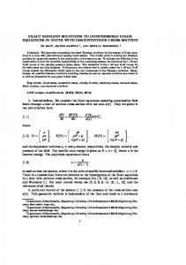
5. Region 5 is a fan region defined by the condition tVt < x − x0 < tVh where the velocity of the head of the wave is again the third eigenvalue, but this time evaluated at the head Vh = v6 + a6 . One uses the expressions for a fan region of a rarefaction wave moving to the right (27,28,29) to calculate the exact solution

Equating these two expression one obtains a trascendental equation for p∗ : " #  ∗  Γ−1 2Γ p 2a A 6 1 1− −(p∗ −p1 ) + +v1 −v6 = 0 p ∗ + B1 Γ − 1 p6 (54) that one solves numerically for p∗ . This information provides the necessary information to construct the solution in the whole domain as described below. The different regions are illustrated in Fig. 3 and the exact solution region by region is as follows. s

1. Region 1 is defined by x − x0 < tVshock , where the velocity of the shock is given by (42) because the shock is traveling to the left:

Vs = v1 − a1

s

pexact vexact ρexact

2Γ   Γ−1 x − x0 Γ−1 2 , v6 − − = p6 Γ + 1 a6 (Γ + 1) t   1 x − x0 2 −a6 + (Γ − 1)v6 + , = Γ+1 2 t 2    Γ−1 2 x − x0 Γ−1 = ρ6 . v6 − − Γ + 1 a6 (Γ + 1) t



6. Region 6 is defined by the condition tVh < x − x0 . The exact solution is given by the initial states at the right chamber.

(Γ + 1)p3 Γ−1 + , 2p1 Γ 2Γ

and the exact solution here reads

pexact = p6 , vexact = v6 , ρexact = ρ6 .

pexact = p1 , vexact = v1 , ρexact = ρ1 . 2. There is no region 2. 3. Region 3 is defined by the condition tVs < x − x0 < tVcontact . Vcontact is the characteristic value (3) evaluated at this region: Vcontact = v3 = v4 = v ∗ . Using (39) explicitly for the density and (52) for the velocity, the solution in this region reads pexact = p3 , vexact = v3 , p1 (Γ − 1) + p3 (Γ + 1) ρexact = ρ1 . p3 (Γ − 1) + p1 (Γ + 1)

An example is shown in Fig. 4 for initial data in Table I. 3.

Case 3: Rarefaction-Rarefaction

A physical situation that provides this scenario is pL = pR , ρL = ρR and −vL = +vR > 0. In this case both, regions 2 and 5 correspond to rarefaction waves. In this particular case since one of the rarefaction waves moves to the left and the other one to the right, we distinguish them using the labels for each of their parts. Again the contact discontinuity defines a relationship between velocity and pressure. In the present case, there

9 t

2

Again, once p∗ is calculated numerically, the solution in all the regions of the domain can be calculated as follows. The first implication is that p3 = p4 = p∗ , and thus v3 and v4 can be calculated using (55) and (56). The different regions are illustrated in Fig. 5.

5 4

3

1

1. Region 1 is defined by the condition x − x0 < tVh,2 , where Vh,2 is the velocity of the head of the wave moving to the left, and is obtained from the characteristic value of such rarefaction wave evaluated at the left interface, that is Vh,2 = v1 − a1 . In this region the gas has not affected the initial state on the left, then the solution is

6

x

1

2

3

4

6

pexact = p1 , vexact = v1 , ρexact = ρ1 .

FIG. 3: Description of the relevant regions for the ShockRarefaction case.

2. Region 2 is a fan region defined by the condition tVh,2 < x − x0 < tVt,2 , where the velocity of the tail Vt,2 is that of the state left behind by the wave, that is Vt,2 = v3 − a3 .

1

1 0.9

0.8

0.8

0.6

0.6

p

ρ

0.7

0.5 0.4

The exact solution is that of a fan region of a rarefaction wave moving to the left (24,25,26)

0.4 0.3 0.2 0.2 0.1 0

0.2

0.4

0.6

0.8

1

0

0.2

0.4

x

0.6

0.8

1

x

0

3

-0.1 2.8 -0.2 2.6

-0.3

2.4

-0.5

2.2

-0.6 -0.7

vexact

2

-0.8 1.8 -0.9 -1

1.6 0

0.2

0.4

0.6

0.8

1

0

x

0.2

0.4

0.6

0.8

1

x

FIG. 4: Exact solution for the Shock-Rarefaction case at time t = 0.25 for the parameters in Table I.

is an expression for v3 in terms of v1 for a rarefaction wave moving to the left given by (19) and another one for v4 in terms of v6 for a rarefaction wave moving to the right (22):

v3 v4

#  Γ−1 p3 2Γ −1 , p1 " #   Γ−1 p4 2Γ 2a6 1− . = v6 − Γ−1 p6

2a1 = v1 − Γ−1

"

(55) (56)

The condition v3 = v4 = v ∗ at the contact discontinuity implies a trascendental equation for p∗ = p3 = p4 : "

2a6 1− Γ−1



"  Γ−1 #  Γ−1 # 2a1 p∗ 2Γ p∗ 2Γ − − 1 +v1 −v6 = 0 p6 Γ−1 p1 (57)

ρexact



2 + Γ+1  2 a1 + = Γ+1  2 = ρ1 + Γ+1

pexact = p1

ε

v

-0.4

2Γ   Γ−1 x − x0 Γ−1 , v1 − a1 (Γ + 1) t  1 x − x0 , (Γ − 1)v1 + 2 t 2   Γ−1 x − x0 Γ−1 . v1 − a1 (Γ + 1) t

3. Region 3 is defined by the condition tVt,2 < x−x0 < tVcontact . The velocity of the contact discontinuity is Vcontact = v3 = v4 = v ∗ according to the eigenvalue (3). In this region p3 = p∗ and v3 = v ∗ are already known from p∗ . Finally, the density is obtained from (13) for an isentropic process like the rarefaction wave for a constant C on both sides of such wave as found in the previous two cases. Thus the solution is

pexact = p3 , vexact = v3 .  1/Γ p3 ρexact = ρ1 , p1 4. Region 4 is defined by the condition tVcontact < x − x0 < tVt,5 , where the velocity of the tail of the wave moving to the right Vt,5 is given by the eigenvalue (4) evaluated at the state left behind the rarefaction wave moving to the right, that is

10 t

Vt,5 = v4 + a4 , where again we point out that v4 = v ∗ and p4 = p∗ are known once p∗ is calculated. The solution is obtained in the same way as for the previous region, but now the wave relates states in regions 4 and 6:

2 4

3

1

6

pexact = p4 , vexact = v4 .  1/Γ p4 , ρexact = ρ6 p6 5. Region 5 is defined by the condition tVt,5 < x − x0 < Vh,5 , where the velocity of the head of the wave moving to the right is Vh,5 = v6 + a6 , and the solution is obtained using the values of the state variables for the fan of a rarefaction wave moving to the right (27,28,29):

x

1

2

3

4

5

6

FIG. 5: Description of the relevant regions for the Rarefaction-Rarefaction case. 0.45 1 0.4

vexact ρexact

0.35 0.8 0.3 0.7

p

0.25

ρ

pexact

2Γ   Γ−1 2 x − x0 Γ−1 = p6 v6 − − , Γ + 1 a6 (Γ + 1) t   1 x − x0 2 −a6 + (Γ − 1)v6 + , = Γ+1 2 t 2   Γ−1  x − x0 Γ−1 2 v6 − − = ρ6 . Γ + 1 a6 (Γ + 1) t



0.9

0.6

0.2

0.5

0.15

0.4

0.1

0.3

0.05

0.2

0 0

0.2

0.4

0.6

0.8

1

0

0.2

0.4

x

0.6

0.8

1

0.6

0.8

1

x

1 1

0.5

0.9

ε

v

0.8

6. Finally, region 6 is defined by the condition Vh,5 < x − x0 . The exact solution is given by the initial values at the chamber on the right because in this region the gas has not been affected yet by the dynamics of the gas:

0

0.7 -0.5 0.6

-1

0.5 0

0.2

0.4

0.6

0.8

1

0

0.2

x

0.4

x

FIG. 6: Exact solution for the Rarefaction-Rarefaction case at time t = 0.25 for the parameters in Table I.

pexact = p6 , vexact = v6 , ρexact = ρ6 .

s

A1 , p 3 + B1

(58)

s

A6 . p 4 + B6

(59)

v3 = v1 − (p3 − p1 )

An example is shown in Fig. 6 for initial data in Table I.

v4 = v6 + (p4 − p6 ) 4.

Case 4: Shock-Shock

A physical situation that provides this scenario corresponds to two streams colliding with opposite directions. We choose in this case pL = pR , ρL = ρR and −vL = +vR < 0. In this case regions 2 and 5 are shock waves. Again the contact discontinuity defines a relationship between velocity and pressure. In the present case there is an expression for v3 in terms of v1 for a shock-wave moving to the left given by (41) and another one for v4 in terms of v6 for a shock-wave moving to the right (43):

The condition v3 = v4 = v ∗ at the contact discontinuity implies a trascendental equation for p∗ = p3 = p4 : s

s A1 A6 ∗ − (p − p1 ) − (p − p6 ) + v1 − v6 = 0. p ∗ + B1 p ∗ + B6 (60) Again, once p∗ is calculated numerically, the solution in all the regions of the domain can be calculated as follows. Immediately one has that p3 = p4 = p∗ and v3 and v4 can be calculated using (58) and (59). ∗

11 t

In this particular case regions 2 and 5 reduce to lines. The solution in each region reads as follows and the regions are illustrated in Fig. 7.

4

3

1. Region 1 is defined by the condition x − x0 < tVs,2 , where the velocity of the shock moving to the leftqVs,2 is given by (42) and reads Vs,2 = v1 − (Γ+1)p3 2p1 Γ

5

2

1

6

Γ−1 2Γ .

+ The solution there is that of a1 the initial values of the variables on the left chamber: x

pexact = p1 , vexact = v1 , ρexact = ρ1 .

4

6

FIG. 7: Description of the relevant regions for the ShockShock case.

2

2.8 2.6

1.8

2.4

1.6

2.2

1.4

2

p

3. Region 3 is defined by the condition tVs,2 < x − x0 < tVcontact , where Vcontact = v3 = v4 = v ∗ . Once (54) is solved one can calculate all the required information. Using (58) for v3 and (39) for ρ3 the solution in this region reads

3

ρ

2. There is no region 2.

1

1.2

1.8 1 1.6 0.8 1.4 0.6

1.2

0.4

1 0

0.2

0.4

0.6

0.8

1

0

0.2

0.4

x

0.6

0.8

1

0.6

0.8

1

x 1.8

1

1.7

1.6

0.5

ε

1.5

v

pexact = p3 , vexact = v3 p1 (Γ − 1) + p3 (Γ + 1) ρexact = ρ1 . p3 (Γ − 1) + p1 (Γ + 1)

0

1.4

1.3

1.2 -0.5

4. Region 4 is defined by tVcontact < x − x0 < tVs,5 , where the velocity of the shock moving to the right q is given by (45) and reads Vs,5 = v6 +

Γ−1 4 a6 (Γ+1)p 2p6 Γ + 2Γ . Finally, using (59) for v4 and (44) for ρ4 the solution in this region reads

1.1

1 -1 0

0.2

5. There is no region 5. 6. Finally region 6 is defined by the condition Vs,5 < x − x0 . The exact solution is given by the initial values at the chamber on the right:

pexact = p6 , vexact = v6 , ρexact = ρ6 . An example is shown in Fig. 8.

0.6

0.8

1

0

0.2

0.4

x

x

FIG. 8: Exact solution for the Shock-Shock case at time t = 0.25 for the parameters in Table I.

III.

pexact = p4 , vexact = v4 , p6 (Γ − 1) + p4 (Γ + 1) . ρexact = ρ6 p4 (Γ − 1) + p6 (Γ + 1)

0.4

RELATIVISTIC SHOCK TUBE

First of all one needs to define a model for the gas. In our case we use the perfect fluid defined because it has no viscosity nor heat transfer, is shear free and is non-compressible. Such system is described by the stress energy tensor T µν = ρ0 huµ uν + pη µν ,

(61)

where ρ0 is the rest mass density of a fluid element, uµ its four velocity, p the pressure, h = 1 + ε + p/ρ0 is the specific enthalpy and η µν are the components of the metric describing Minkowski space-time. The set of relativistic Euler equations is obtained from the local conservation of the rest mass and the local conservation of the stress energy tensor of the fluid, which are respectively

12 that all quantities describing the fluid depend on the variable ξ = (x − x0 )/t. In order to explore the change of all physical quantities along the straight line ξ, we define the useful change on the derivative operators

(ρ0 uµ ),µ = 0, (T µν ),ν = 0, 1 1−v i vi

where uµ = W (1, v x , 0, 0) and W = √

is the

Lorentz factor and v x is the Eulerian velocity of the fluid elements. It is possible to arrange these equations as a flux balance set of equations as in the Newtonian case ∂t u + ∂x F(u) = 0,

The flux balance equations are explicitly: ∂t D + ∂x (Dv) = 0, ∂t S + ∂x (Sv + p) = 0, ∂t τ + ∂x S = 0.

∂x p = −Dda (hW v), ∂t p = Dda (hW ),

where we have used the rest mass conservation law to simplify the expressions. From (69) we obtain for the advective derivative da = 1t (ξ − v)d/dξ, for which we will use d := d/dξ from now on. With this in mind we obtain from (70,71) the differential equation

(64) (65) (66)

v ± cs . 1 ± vcs

(67)

Each of the characteristic values (67) may correspond to eigenvectors with different properties exactly as in the Newtonian case, that is, λ0 corresponds to a contact discontinuity, whereas the eigenvalues λ± may correspond to rarefaction or shock waves. The shock tube problem in this case is defined as in the Newtonian case:

u=

(

uL , x < x0 uR , x > x0 .

(72)

On the other hand, the change of variable in (64) from t, x to ξ implies (v − ξ)dρ + ρW 2 (1 − vξ)dv = 0.

(73)

and from equations (72) and (73) we obtain a relation between the density and pressure

The eigenvalues of the Jacobian matrix of this system of equations are λo = v, λ± =

(70) (71)

(v − ξ)ρhW 2 dv + (1 − ξv)dp = 0. (63)

(69)

Using the advective derivative da = ∂t +v∂x , we obtain the expressions

(62)

where conservative variables are defined by u = (D, S x , τ )T and the resulting fluxes are F = (Dv, Sv + p, S), where we assume that specifically v = v x and S = S x , since we are only considering one spatial dimension. The conservative variables are defined in terms of the primitive ones as follows D = ρ0 W, S = ρ0 hW 2 v, τ = = ρ0 hW − p.

1 1 ∂t = − ξ∂ξ , ∂x = ∂ξ . t t

dp = h



v−ξ 1 − vξ

2

dρ.

(74)

Since the process along ξ is isentropic [6] the sound speed ∂p is c2s = h1 ∂ρ |s , which combined with the previous expression implies the speed of sound v−ξ . cs (v, ξ) = 1 − vξ

(75)

Besides, we can find a useful expression for an isentropic process using p = KρΓ (we are using a politropic equation of state).

(68) cs =

Next we describe the treatment of each of the wave or discontinuities that develop during the evolution.

s

Γp . ρh

(76)

From system (67) we obtain the speed of sound in terms of the eigenvalues of the Jacobian matrix A.

Rarefaction Waves

Rarefaction waves are self-similar solutions of the flow equations [4]. They are self-similar solutions in the sense

cs =

(

−(v − λ+ )/(1 − vλ+ ) (v − λ− )/(1 − vλ− )

if ξ = λ+ , if ξ = λ− .

(77)

13 Comparing with (75) we find that cs (v, λ+ ) is the speed of sound for a rarefaction wave traveling to the right and cs (v, λ− ) for a wave traveling to the left. According to this equation we get from (73) that W 2 dv ±

cs dρ = 0. ρ

(78)

Here the + sign refers to the wave traveling to the left and the − sign when it travels to the right. From this equation we obtain the Riemann invariant because this differential equation is valid along a straight line along the x − t plane, as long as it is not a shock. Integrating the first term of (78) we obatain 1 1+v ln ± 2 1−v

cs dρ = constant. ρ

Z

(79)

In order to calculate the integral we use the definition of the sound speed and the polytropic equation of state p = KρΓ , from which we obtain

c2s (ρ) =

KΓ(Γ − 1)ρΓ−1 , Γ − 1 + KΓρΓ−1

1−Γ KΓ

Γ−1
Γ−1 p Γ K

.

(81)

Conversely, if the speed of sound is known one can calculate the density using (80):

Then the integral can be written as Z

cs dρ = ρ

Z



cs KΓ



1 1 − 2 cs Γ−1

1  Γ−1

1 + vR ± 1 + vL ± AL = A . 1 − vL 1 − vR R

dρ dcs . (83) dcs

+ (1 + vL )A+ L − (1 − vL )AR +. (1 + vL )A+ L + (1 − vL )AR

(88)

Analogously when the wave is moving to the right we expect to account with information on the state to the right. Then we can express the velocity on the left in terms of the variables on the state at the right and A−

vL =

− (1 + vR )A− R − (1 − vR )AL −. (1 + vR )A− R + (1 − vR )AL

1.

(89)

The fan

The fan is the region where the rarefaction takes place, propagating with velocity either λ+ if the wave is moving to the right or λ− when moving to the left. The fan will be bounded by two values of ξ corresponding to the head and the tail of the wave: (L,R)

Integrating by parts and using (79) we find the useful constraint

ξh =

vL,R ± cs

√  Γ − 1 + cs 1 1+v 1 √ ln ln ± = constant, 2 1 − v (Γ − 1)1/2 Γ − 1 − cs (84) which in turn simplifies as follows

ξt =

vR,L ± cs

1+v ± A = constant, 1−v

(87)

Assuming that when the wave is propagating to the left we account with information from the left state, we can calculate the velocity of the fluid on the region at the right from the wave in terms of the state variables on the state at the left and A+ :

(82)

s

(86)

Equation (85) is valid only across straight lines arising from the origin (x0 , t = 0) and evolving along ξ = (x − x0 )/t inside the rarefaction zone. For this family of straight lines the Riemann invariant is the same. This allows us to relate any two different states in the rarefaction zone, particularly we are going to take the states L and R as the states just next to the left and to the right from the rarefaction wave.

vR =

+1

1 ρ= h . 1  i Γ−1 1 1 KΓ c2 − Γ−1

√ ±2(Γ−1)−1/2 Γ − 1 + cs A = √ . Γ − 1 − cs ±

(80)

or in terms of the pressure instead of the density the speed of sound reads c2s (p) =

where A± is

(85)

(L,R)

1 ± vcs

(90)

,

(91)

(R,L)

(R,L)

1 ± vcs

,

where the − sign applies to waves traveling to the left and + when the wave moves to the right. In order to construct the solution inside the fan, we use the constraint (87). We have two cases according to the direction of the rarefaction wave. If the rarefaction wave travels to left we use

14

1 + vL + 1 + vR + A − A =0 1 − vL L 1 − vR R

(92)

and solve the equation for vR . When the rarefaction wave travels to right we use 1 + vL − 1 + vR − A − A = 0, 1 − vL L 1 − vR R

(93)

DL vL − DR vR = Vs (DL − DR ), (96) SL vL + pL − (SR vR + pR ) = Vs (SL − SR ), (97) SL − SR = Vs (τL − τR ). (98) The subindices (L, R) represent two arbitrary states at left and at the right from the shock. These equations can be written in the reference rest frame of the shock by considering a Lorentz transformation, that is

and solve the equation for vL . We calculate in each case A± using (86) in the appropriate region

A± (L,R)

"√ #±2(Γ−1)−1/2 Γ − 1 + c± s,(L,R) = √ , Γ − 1 − c± s,(L,R)

(94)

where the sound speed is given by (75) and (77)

c± s,(L,R) = ±

v(L,R) − ξ , 1 − v(L,R) ξ

(99) (100) (101)

where the hatted quantities are evaluated at the rest Vs −v(L,R) ˆ (L,R) = frame of the shock. Here vˆ(L,R) = 1−V ,D s v(L,R) ˆ L,R , Sˆ(L,R) = ρ(L,R) h(L,R) W ˆ2 ρ(L,R) W vˆ(L,R) and (L,R)

ˆ (L,R) = W (95)

where the + sign is used when the wave moves to the left and − when moving to the right. Finally since we are in the rarefaction zone we can express a point (x, t) with ξ = (x − x0 )/t in (95) and using this expression in (94) and substituting into (92) or (93) depending on the direction of propagation we finally obtain a trascendental equation for the velocity v(L,R) . We assume that if the wave moves to the left we know the variables on the state to the left L and ignore those of the state to the right R and viceversa. Then we look for a solution of vL when the wave moves to the left and of vR when moving to the right. Instead of looking for a closed solution to this equation we solve it numerically to obtain v(L,R) assuming we know v(R,L) . Once v(L,R) is calculated we can substitute back, and using equation (95) obtain the sound speed; next, using (82) obtain the density ρ; finally with the help of the EOS we can calculate the pressure p = KρΓ . This completes the solution in the fan region. The particular cases described later illustrate how to implement this procedure.

B.

ˆ L vˆL = D ˆ R vˆR , D SˆL vˆL + pL = SˆR vˆR + pR , SˆL = SˆR ,

Shock Waves

Shocks require the use of the relativistic RankineHugoniot jump conditions [ρ0 uµ ]nµ = 0 and [T µν ]nν = 0 across the shock [6], where nµ = (−Vs Ws , W s, 0, 0) is a normal vector to the shock’s front, Ws is the shock’s Lorentz factor and Vs is the speed of the shock. Here we have used the notation [F ] = FL − FR , where FL and FR are the values of the function F at both sides of the shock’s surface. These conditions reduce to the following system of equations, in terms of primitive and conservative variables, as

q

1 . 2 1−ˆ v(L,R)

From (99), we can introduce the invariant relativistic mass flux across the shock as j = Ws DL (Vs − vL ) = Ws DR (Vs − vR ), where Ws = √

1 . 1−Vs2

(102)

It is important to point out that

when the shock moves to the right the mass flux is positive j > 0, whereas when the shock moves to the left it has to be negative j < 0. Now, using the expression for the mass flux (102) into the Rankine-Hugoniot conditions (96, 97, 98) we can obtain the following system of equations in terms of a combination of primitive and conservative variables vL − vR pL − pR vL pL − vR pR

  1 1 j , − = − Ws DL DR   j SR SL = , − Ws DL DR   τR τL j . − = Ws DL DR

(103) (104) (105)

Considering the shock is moving to the right and thus that the state R is known, we will write an expression for the velocity vL in terms of the state variables R and also in terms of j, Vs and pL . In order to do this, we rewrite expressions (104) and (105) using the definitions for the conservative variables in terms of the primitive variables (63) as follows Ws vR (pL − pR ) = hL WL − hR WR , (106) jvL vL pL Ws (107) (vL pL − vR pR ) = hL WL − j ρL WL pR − hR WR + . ρR WR

15 Subtracting these expressions and dividing by pL we get   vR pR Ws 1 pR vL − = (108) − + j pL vL vL pL   pR 1 hR WR vR −1 + − . pL vL pL ρR WR ρL WL Inserting this into (103) we finally obtain an expression for the velocity vL

vL =

hR WR vR +

Ws j (pL

hR WR + (pL − pR )



− pR )

Ws vR j

+

.

1 ρR WR

vR =

Ws j (pR

hL WL + (pR − pL )



− pL )

Ws vL j

+

1 ρL WL

,

(110)

where the condition j < 0 has to be satisfied. In order to obtain the shock velocity Vs , we start form the mass flux conservation across the shock (102), which relates the shock p velocity with the mass flux. Substituting Ws = 1/ 1 − Vs2 , it is possible to solve the resulting quadratic equation and obtain the two roots for the shock velocity

Vs Vs

p ρ2R WR2 vR + j 4 + j 2 ρ2R = , ρ2R WR2 + j 2 p ρ2L WL2 vL − j 4 + j 2 ρ2L = , ρ2L WL2 + j 2

(112)

ρL hL (Vs − vL )2 ρR hR (Vs − vR )2 − 2 + V 2 v2 2 + V 2 v2 = 1 − Vs2 − vL 1 − Vs2 − vR s L s R − (pL − pR ). (113) 1 q 2 2 +Vs2 v(L,R) 1−Vs2 −v(L,R)

ing form

=

√

1−Vs2

1 q

2 1−v(L,R)

=

the last equation takes the follow-

(115)

where the positive root corresponds to a shock moving to the right whereas the negative root to a shock moving to the left. Another useful expression comes from equation (101), which can be rewritten directly in the form

ˆ R, ˆ L = hR W hL W

(116)

which combined with equation (115) implies

h2L − h2R = (pL − pR )

(111)

which correspond respectively to a shock moving to the right and to the left. The signs of the quadratic formula are chosen such that they are physically possible, that is, for the case of a shock moving to the right j > 0 we use (111) and for a shock moving to the left j < 0 we use (112) [3]. In order to solve completely the problem across the shock, we first express equation (100) as

Considering that Ws W(L,R)

−(pL − pR ) , j2 =  hL hR ρL − ρR

(109)

When the shock moves to the left and the state L is known, the velocity on the state to the right is hL WL vL +

ρL hL Ws2 WL2 (Vs −vL )2 −ρR hR Ws2 WR2 (Vs −vR )2 = −(pL −pR ). (114) As we can see from this equation, the definition of the conserved mass flux is present, then using equation (102) in this last equation, we obtain a useful expression for the square of the flux



hL hR + ρL ρR



.

(117)

This last equation is commonly called the Taub’s adiabat. Moreover equations (115), (116) and (117) are known as relativistic Taub’s junction conditions for shock waves [6, 7]. Finally, in order to obtain the density ρL and pressure pL for a shock moving to the right in terms of the variables in the region to the right, we consider the definition of the specific internal enthalpy and that the fluid obeys and ideal gas equation of state. With these assumptions equation (117) can be rewritten in the form

1 σ [pL (2σ − 1) + pR ] + 2 [p2L (σ − 1) + pL pR ] = ρL ρL σ 1 [pR (2σ − 1) + pL ] + 2 [p2R (σ − 1) + pL pR ],(118) ρR ρR where σ = reads

Γ Γ−1 .

The solution for the quadratic equation

16

where ζL =

p [pL (2σ − 1) + pR ]2 + 4ζL σ[p2L (σ − 1) + pL pR ] , 2σ[p2L (σ − 1) + pL pR ] p −[pR (2σ − 1) + pL ] ± [pR (2σ − 1) + pL ]2 + 4ζR σ[p2R (σ − 1) + pR pL ] = , 2σ[p2R (σ − 1) + pR pL ]

−[pL (2σ − 1) + pR ] ± 1 = ρL

(119)

1 ρR

(120)

1 ρR [pR (2σ

− 1) + pL ] + ρσ2 [p2R (σ − 1) + pL pR ], R

and ζR = ρ1L [pL (2σ − 1) + pR ] + ρσ2 [p2L (σ − 1) + pR pL ]. L A physically acceptable solution requires ρ > 0, which restricts the sign to be positive one in both cases.

v3 =

+ (1 + v1 )A+ 1 − (1 − v1 )A3 +. (1 + v1 )A+ 1 + (1 − v1 )A3

(122)

where according to (94) C.

Contact Wave

The equations describing the jump conditions (96,97,98) admit the solution using Vs = vR = vL = λo = Vcontact where vR and vL are the values of the velocity of the fluid at the right and at the left from the contact discontinuity. This represents the contact wave traveling along the line x − x0 = λ0 t. Then (96) is trivial and (97) reads (SL − SR )Vs + pL − pR = (SL − SR )Vs ,

(121)

which implies pR = pL and equation (98) is satisfied. We are now in the position of analyzing each of the possible combinations of shock and rarefaction waves in a Riemann problem. We then proceed in the same way as in the Newtonian case studying each combination. D.

The four different cases

In what follows, as we did for the Newtonian case, we present the four combinations of rarefaction and shock waves associated to the relativistic Riemann problem. We illustrate each case with a particular set of parameters contained in Table II. 1.

Case 1: Rarefaction-Shock

The contact wave conditions are v3 = v4 = v ∗ and p3 = p4 = p∗ . The velocity in region 3 is given by equation (88) that provides the velocity on the state at the right from a rarefaction wave moving to the left:

A+ (1,3)

"√ #+2(Γ−1)−1/2 Γ − 1 + c+ s,(1,3) = √ . Γ − 1 − c+ s,(1,3)

(123)

p p1 Γ and Γp1 /(ρ1 h1 ), h1 = 1+ ρ1 (Γ−1) Here c+ s,1 := cs (p1 ) = + cs,3 := cs (p3 ) is given by equation (81) v u u c+ s,3 (p3 ) = t

Γ−1 KΓ

Γ−1
1−Γ p3 Γ K

,

K=

+1

p1 , ρΓ1

(124)

where we remind the reader that in the rarefaction region the polytopic constant remains the same during the process, that is, it is the same in regions 1, 2 and 3. On the other hand the velocity of the gas in region 4 corresponds to the velocity on the state at the left of a shock moving to the right (109)

v4 =

h6 W6 v6 +

Ws,5 j (p4

h6 W6 + (p4 − p6 )



− p6 )

Ws,5 v6 j

+

1 ρ6 W6

,

(125)

q 2 is the Lorentz factor of the where Ws,5 = 1/ 1 − Vs,5 shock, where we use the subindex 5 in order to denote the shock occurring in region 5. In order to obtain v4 in terms of p4 we need to perform the following steps: • The rest mass density ρ4 is given in terms of p4 and other known information can be expressed using (119) as

p −[p4 (2σ − 1) + p6 ] + [p4 (2σ − 1) + p6 ]2 + 4ζ4 σ[p24 (σ − 1) + p4 p6 ] 1 = , ρ4 2σ[p24 (σ − 1) + p4 p6 ] σ Γ 1 [p6 (2σ − 1) + p4 ] + 2 [p26 (σ − 1) + p4 p6 ], where σ = . ζ4 = ρ6 ρ6 Γ−1

(126) (127)

17 Case pL pR vL vR ρL ρR Rarefaction-Shock 13.33 0 0 0 10 1 Shock-Rarefaction 0 13.33 0.0 0.0 1 10 Rarefaction-Rarefaction 0.05 -0.05 -0.2 0.2 0.1 0.1 Shock-Shock 3.333e-9 -3.333e-9 0.999999 0.999999 0.001 0.001 TABLE II: Initial data for the four different cases. We choose the spatial domain to be x ∈ [0, 1] and the location of the membrane at x0 = 0.5. In all cases we use Γ = 4/3.

• Once ρ4 is given in terms of p4 it is possible to compute the enthalpy in region 4 as h4 = 1 + σ ρp44 . • Then equation (115) reads j2 = −

(p4 − p6 ) , h6 h4 ρ4 − ρ6

1. Region 1 is defined by the condition x − x0 < tξh , where according to (90) ξh is the velocity of the head of the rarefaction wave traveling to the left v1 −cs,1 ξh = 1−v . The values of the physical variables 1 cs,1 are known from the initial conditions:

(128) pexact = p1 , vexact = v1 , ρexact = ρ1 .

where h6 = 1 + σ pρ66 . Something to remember here is the fact that as the shock moves to the right, we consider j to be the positive square root. • Once j is obtained, the shock velocity can be found from expression (111) as

Vs,5

p ρ26 W62 v6 + |j| j 2 + ρ26 . = j 2 + ρ26 W62 1 2 1−Vs,5

• Finally one calculates Ws,5 = √

(129)

2. Region 2 is defined by the condition tξh < x − x0 < tξt , where according to (91) ξt is the characteristic value again, but this time evaluated at the tail of v3 −cs,3 the rarefaction wave, that is ξt = 1−v . In order 3 cs,3 to compute v2 we use (92)

and in this

1 + v1 + 1 + v2 + A − A (v2 ) = 0 1 − v1 1 1 − v2 2

way v4 in terms of p4 and the known state in region 6 using (125).

According to the contact discontinuity condition v3 = v4 = v ∗ , we equate (122) and (125) and obtain a transcendental equation for p∗ : + ∗ (1 + v1 )A+ 1 − (1 − v1 )A3 (p ) − + ∗ (1 + v1 )A+ 1 + (1 − v1 )A3 (p )

h6 W6 v6 +

Ws ∗ j (p

h6 W6 + (p∗ − p6 )



− p6 )

Ws v6 j

+

1 ρ6 W6

 = 0,

(130)

which has to be solved using a root finder. Once this equation is solved, p3 and p4 are automatically known and v3 and v4 can be calculated using (122) and (125), respectively. It is possible to calculate ρ3 using the fact that in the rarefaction zone the process is adiabatic and then ρ3 = ρ1 (p3 /p1 )1/Γ . On the other hand we can also calculate ρ4 using (126). With this information it is already possible to construct the solution in the whole domain. Up to this point we account with the known initial states (p1 , v1 , ρ1 ) and (p6 , v6 , ρ6 ), the solution in regions 3 and 4 given by (p3 , v3 , ρ3 ) and (p4 , v4 , ρ4 ), and Vs,5 which represents the velocity of propagation of the shock 5. The exact solution region by region is described next.

(131) (132) (133)

(134)

considering equations (76), (94) and (95) as follows

A+ (1,2) =

"√

c+ s,1

s

=

c+ s,2 =

√

Γ − 1 + c+ s,(1,2) Γ − 1 − c+ s,(1,2)

#+2(Γ−1)−1/2

, (135)



(136)

p1 Γp1 , h1 = 1 + ρ1 h 1 ρ1

v2 − ξ 1 − v2 ξ

⇒ v2 =



Γ Γ−1

ξ + c+ s,2

1 + c+ s,2 ξ

.

(137)

where ξ = (x − x0 )/t. In this way, equation (134) is transcendental and has to be solved equivalently for v2 or for c+ s,2 using a root finder for each point of region 2. We recommend solving for c+ s,2 and then construct v2 using (137). Finally we calculate ρ2 using equation (82): 1 ρ2 =   KΓ (c+1 )2 − s,2

1 Γ−1

, 1  Γ−1

K=

p1 . ρΓ1

(138)

18 Finally we obtain p2 using the fact that in the process K is constant

p2 = p1



ρ2 ρ1

Γ

.

(139)

3. Region 3 is defined by the condition tξt < x − x0 < tVcontact , where Vcontact = λo = v3 = v4 . The solution there reads

2.

This is pretty much the previous case, except that one has to be careful at using the correct signs and conditions. We then start again with the contact wave conditions v3 = v4 = v ∗ and p3 = p4 = p∗ . The velocity of the gas in region 3 corresponds to the velocity on the state at the right from a shock moving to the left (110)

v3 = pexact = p3 , vexact = v3 , ρexact = ρ3 .

(140) (141) (142)

4. Region 4 is defined by the condition tVcontact < x − x0 < tVs,5 , where Vs,5 is given by (129) and explicitly

Case 2: Shock-Rarefaction

h1 W1 v1 +

Ws,2 j (p3

h1 W1 + (p3 − p1 )



− p1 )

Ws,2 v1 j

+

1 ρ1 W1

,

(149)

q 2 is the Lorentz factor of the where Ws,2 = 1/ 1 − Vs,2 shock. In order to obtain v3 in terms of p3 and other known information we need to perform the following steps: 14

10

12 8 10

6

p

(143) (144) (145)

ρ

pexact = p4 , vexact = v4 , ρexact = ρ4 .

8

6 4 4 2 2

0

0 0

0.2

0.4

0.6

0.8

1

0

0.2

0.4

x

5. There is no region 5. Only the shock traveling with speed Vs,5 .

0.8

1

0.6

0.8

1

0.6 1.5 0.5

0.4

ε

v

6. Region 6 is defined by tVs,5 < x − x0 . In this region the solution is simply

0.6

x 2

0.7

1

0.3

0.2

0.5

0.1

0

0 0

0.2

0.4

0.6

0.8

1

0

0.2

x

pexact = p6 , vexact = v6 , ρexact = ρ6 .

0.4

x

(146) (147) (148)

FIG. 9: Exact solution for the Rarefaction-Shock case at time t = 0.35 for the parameters in Table II.

As an example we show in Fig. 9 the primitive variables at t = 0.35, for the initial parameters in Table II.

• The rest mass density is given in terms of p3 using the expression (120) as

p 1 −[p3 (2σ − 1) + p1 ] + [p3 (2σ − 1) + p1 ]2 + 4ζ3 σ[p23 (σ − 1) + p3 p1 ] = , ρ3 2σ[p23 (σ − 1) + p3 p1 ] 1 σ Γ ζ3 = [p1 (2σ − 1) + p3 ] + 2 [p21 (σ − 1) + p3 p1 ], where σ = . ρ1 ρ1 Γ−1

• Once ρ3 is given in terms of p3 it is possible to compute the enthalpy in region 3 as h3 = 1 + σ ρp33 .

• Then from equation (115) we obtain

j2 = −

(p3 − p1 ) , h1 h3 ρ3 − ρ1

(150) (151)

(152)

where h1 = 1 + σ pρ11 . As the shock is moving to

19 the left we consider the negative root of the above expression for j. • Once j is obtained, the shock velocity can be found from expression (112) in terms of p3 as

Vs,2

p ρ21 W12 v1 − |j| j 2 + ρ21 . = j 2 + ρ21 W12 1 2 1−Vs,2

• Finally one calculates Ws,2 = √

pexact = p1 , vexact = v1 , ρexact = ρ1 .

(153) and in this

way v3 in terms of p3 and the known state in region 1 using (149).

The velocity in region 4 is given by equation (89) that provides the velocity on the state at the left from a rarefaction wave moving to the right: v4 =

1. Region 1 is defined by the condition x − x0 < tVs,2 , where Vs,2 is given by (153) and the solution there is that of the initial state on the left chamber

− (1 + v6 )A− 6 − (1 − v6 )A4 −, (1 + v6 )A− 6 + (1 − v6 )A4

2. There is no region 2. Only the shock traveling with speed Vs,2 . 3. Region 3 is defined by the condition tVs,2 < x − x0 < tVcontact , where Vcontact = λo = v3 = v4 . The solution is

pexact = p3 , vexact = v3 , ρexact = ρ3 .

(154)

where following (94) "√ #−2(Γ−1)−1/2 Γ − 1 + c− s,(4,6) − A(4,6) = √ . (155) Γ − 1 − c− s,(4,6) p p6 Γ and Γp6 /(ρ6 h6 ), h6 = 1+ ρ6 (Γ−1) Here c− s,6 := cs (p6 ) = c− := c (p ) is given by equation (81) s 4 s,4 v u u c− s,4 (p4 ) = t

Γ−1 KΓ

Γ−1
1−Γ p4 Γ K

,

K=

+1

p6 . ρΓ6

pexact = p4 , vexact = v4 , ρexact = ρ4 .

Ws ∗ j (p

h1 W1 + (p∗ − p1 )



− p1 )

Ws v1 j

+

1 ρ1 W1

 = 0,

(164) (165) (166)

5. Region 5 is defined by the condition tξt < x − x0 < tξh , where according to (90) ξh is the velocity of the head of the rarefaction wave traveling to the right v6 +cs,6 . In order to compute v5 we use (93) ξh = 1+v 6 cs,6

− ∗ (1 + v6 )A− 6 − (1 − v6 )A4 (p ) − − ∗ (1 + v6 )A− 6 + (1 − v6 )A4 (p )

h1 W1 v1 +

(161) (162) (163)

4. Region 4 is defined by the condition tVcontact < x − x0 < tξt , where according to (91) ξt is the characteristic value again, but this time evaluated at the tail of the rarefaction wave, that is ξt = v4 +cs,4 1+v4 cs,4 . The solution in this region is

(156)

because K is the same in regions 4 and 6. We obtain a transcendental equation for p∗ using the contact discontinuity condition v3 = v4 = v ∗ , and equate (149) and (154):

(158) (159) (160)

1 + v6 − 1 + v5 − A − A (v5 ) = 0, 1 − v6 6 1 − v5 5 (157)

which has to be solved using a root finder. Once this equation is solved, p3 and p4 are automatically known and v3 and v4 can be calculated using (149) and (154), respectively. It is possible to calculate ρ4 using the fact that in the rarefaction zone the process is adiabatic and then ρ4 = ρ6 (p4 /p6 )1/Γ . We can also calculate ρ3 using (150). With this information it is already possible to construct the solution in the whole domain. Up to this point we have the known initial states (p1 , v1 , ρ1 ) and (p6 , v6 , ρ6 ), the solution in regions 3 and 4 given by (p3 , v3 , ρ3 ) and (p4 , v4 , ρ4 ), and Vs,2 which represents the velocity of propagation of the shock 2. The exact solution region by region is described next.

(167)

whoch requires the information in (76), (94) and (95):

A− (5,6) c− s,6

#−2(Γ−1)−1/2 "√ Γ − 1 + c− s,(5,6) = √ , (168) Γ − 1 − c− s,(5,6) s   p6 Γ Γp6 (169) , h6 = 1 + = ρ6 h 6 ρ6 Γ − 1

c− s,5 =

v5 − ξ 1 − v5 ξ

⇒ v5 =

ξ − c− s,5

1 − c− s,5 ξ

.

(170)

where ξ = (x − x0 )/t. In this way, equation (167) is transcendental and has to be solved equivalently

20 for v5 or for c− s,5 using a root finder for each point of region 5. We recommend solving for c− s,5 and then construct v5 using (170). Finally we calculate ρ5 using equation (82):

v3 =

+ (1 + v1 )A+ 1 − (1 − v1 )A3 , + (1 + v1 )A1 + (1 − v1 )A+ 3

(176)

where according to (94) ρ5 = 

1 KΓ



1 2 (c− s,5 )

−

1 Γ−1

, 1  Γ−1

p6 K = Γ, ρ6

(171) A+ (1,3)

since K is the same in regions 5 and 6, and by the same reason we obtain p5 using

p5 = p6



ρ5 ρ6

Γ

.

(172)

6. Region 6 is defined by tξh < x − x0 . In this region the solution is simply

pexact = p6 , vexact = v6 , ρexact = ρ6 .

(173) (174) (175)

As an example we show in Fig. 10 the primitive variables at t = 0.35 for the initial data in Table II.

v u u c+ s,3 (p3 ) = t

v4 =

p

ρ

8

6

K

,

K=

+1

p1 . ρΓ1

(178)

− (1 + v6 )A− 6 − (1 − v6 )A4 , − (1 + v6 )A6 + (1 − v6 )A− 4

(179)

where according to (94)

A− (4,6)

10

6

Γ−1 KΓ

Γ−1
1−Γ p3 Γ

On the other hand the velocity of the gas in region 4 corresponds to the velocity on the state at the left of a rarefaction wave moving to the right (89)

12 8

(177)

p p1 Γ Γp1 /(ρ1 h1 ), h1 = 1+ ρ1 (Γ−1) and Here c+ s,1 := cs (p1 ) = + cs,3 := cs (p3 ) is given by equation (81)

14

10

"√ #+2(Γ−1)−1/2 Γ − 1 + c+ s,(1,3) = √ . Γ − 1 − c+ s,(1,3)

"√ #−2(Γ−1)−1/2 Γ − 1 + c− s,(4,6) = √ , Γ − 1 − c− s,(4,6)

(180)

4

and the speed of sound in region 4 is given by

4 2 2

0

0 0

0.2

0.4

0.6

0.8

1

0

0.2

0.4

x

0.6

0.8

1

x

v u u c− s,4 (p4 ) = t

0 2 -0.1

-0.2

1.5

ε

v

-0.3

-0.4

1

-0.5 0.5 -0.6

-0.7 0 0

0.2

0.4

0.6

x

0.8

1

0

0.2

0.4

0.6

0.8

1

x

FIG. 10: Exact solution for the Shock-Rarefaction case at time t = 0.35 for the parameters in Table II.

3.

Case 3: Rarefaction-Rarefaction

In this case the transcendental equation for the pressure at the contact discontinuity is given again by the condition v3 = v4 where both velocities are constructed using the information of the unknown state aside rarefaction waves. The velocity in region 3 is given by equation (88) for the velocity on the state at the right from a rarefaction wave moving to the left:

Γ−1 KΓ

Γ−1
1−Γ p4 Γ K

,

K=

+1

p6 . ρΓ6

(181)

Then using the contact discontinuity condition v3 = v4 = v ∗ , we equate (176) and (179) and obtain a transcendental equation for p∗ : + ∗ (1 + v1 )A+ 1 − (1 − v1 )A3 (p ) − + ∗ (1 + v1 )A1 + (1 − v1 )A+ 3 (p )

− ∗ (1 + v6 )A− 6 − (1 − v6 )A4 (p ) = 0, − ∗ (1 + v6 )A− 6 + (1 − v6 )A4 (p )

(182)

which has to be solved using a root finder. Once this equation is solved, p3 and p4 are automatically known and v3 and v4 can be calculated using (176) and (179), respectively. As in the previous two cases, it is possible to calculate ρ3 and ρ4 using the fact that in the rarefaction zone the process is adiabatic and then ρ3 = ρ1 (p3 /p1 )1/Γ and ρ4 = ρ6 (p4 /p6 )1/Γ . Thus we have the known initial states (p1 , v1 , ρ1 ), (p6 , v6 , ρ6 ) and

21 the solution in regions 3 and 4 given by (p3 , v3 , ρ3 ) and (p4 , v4 , ρ4 ). The solution in each of the fan regions aside the rarefaction zones has to be constructed in terms of the position and time ξ = (x − x0 )/t as described below for regions 2 and 5. 1. Region one is defined by the condition x−x0 < tξh2 , where according to (90) ξh2 is the velocity of the head of the rarefaction wave traveling to the left v1 −cs,1 ξh2 = 1−v . The values of the physical variables 1 cs,1 are known from the initial conditions:

pexact = p1 , vexact = v1 , ρexact = ρ1 .

(183) (184) (185)

2. Region 2 is defined by the condition tξh2 < x−x0 < tξt2 , where according to (91) ξt2 is the characteristic value again, but this time evaluated at the tail of v3 −cs,3 the rarefaction wave, that is ξt2 = 1−v . In 3 cs,3 order to compute v2 we use (92) 1 + v1 + 1 + v2 + A − A (v2 ) = 0, 1 − v1 1 1 − v2 2

c+ s,1

v2 − ξ 1 − v2 ξ

⇒ v2 =

ξ + c+ s,2

1+

. c+ s,2 ξ

(189)

where ξ = (x − x0 )/t. In this way, equation (186) is transcendental and has to be solved equivalently for v2 or for c+ s,2 using a root finder for each point of region 2. We solve for c+ s,2 and construct v2 using (189). Finally we calculate ρ2 using equation (82):

ρ2 = 

1 KΓ



1 2 (c+ s,2 )

−

1 Γ−1

, 1  Γ−1

(192) (193) (194)

4. Region 4 is defined by the condition tVcontact < x − x0 < tξt5 , where ξt5 is the third characteristic value calculated at the tail of rarefaction moving to v4 +cs,4 . In the right, and according to (91) ξt5 = 1+v 4 cs,4 this region thus pexact = p4 , vexact = v4 , ρexact = ρ4 .

(195) (196) (197)

5. Region 5 is defined by the condition tξt5 < x−x0 < v6 +cs,6 tξh5 , where ξh5 = 1+v according to (90). In 6 cs,6 order to compute v5 we use (93) 1 + v5 − 1 + v6 − A (v5 ) − A = 0, 1 − v5 5 1 − v6 6

(198)

where according to (76), (94) and (95)

"√ #+2(Γ−1)−1/2 Γ − 1 + c+ s,(1,2) = √ , (187) Γ − 1 − c+ s,(1,2) s   Γp1 p1 Γ (188) , h1 = 1 + = ρ1 h 1 ρ1 Γ − 1

c+ s,2 =

pexact = p3 , vexact = v3 , ρexact = ρ3 .

(186)

where using (76), (94) and (95)

A+ (1,2)

3. Region 3 is defined by the condition tξt2 < x−x0 < tVcontact , where Vcontact = λo = v3 = v4 . The solution there reads

p1 K = Γ. ρ1

(190)

A− (5,6) c− s,6

#−2(Γ−1)−1/2 "√ Γ − 1 + c− s,(5,6) , (199) = √ Γ − 1 − c− s,(5,6) s   p6 Γ Γp6 , (200) , h6 = 1 + = ρ6 h 6 ρ6 Γ − 1

c− s,5 = −

v5 − ξ 1 − v5 ξ

⇒ v5 =

ξ − c− s,5

1 − c− s,5 ξ

,

(201)

where ξ = (x − x0 )/t. Again (198) is a transcen− dental equation either for v5 or for c− s,5 . Once cs,5 has been calculated use (201) to construct v5 or directly solve (198) for v5 . It is possible to calculate ρ5 using (82): 1 ρ5 =   KΓ (c−1 )2 − s,5

1 Γ−1

, 1  Γ−1

K=

p6 , ρΓ6

(202)

and finally the pressure

Finally we obtain p2 using p2 = p1



ρ2 ρ1

Γ

.

(191)

p5 = p6



ρ5 ρ6

Γ

.

(203)

22 6. Region 6 is defined by tξh5 < x − x0 . In this region the solution is simply

pexact = p6 , vexact = v6 , ρexact = ρ6 .

(204) (205) (206)

4.

Shock-Shock

We proceed as always, by establishing a relationship between the velocity in regions 3 and 4. We start by expressing v3 as the velocity of the gas on a region at the right from a shock moving to the left, that is, according to (110)

As an example we show in Fig. 11 the primitive variables at t = 0.25, for the initial parameters in Table II. 0.105 0.05

v3 =

0.1

0.095 0.045 0.09

0.04

ρ

p

0.085

h1 W1 v1 +

Ws,2 j2 (p3

h1 W1 + (p3 − p1 )

0.08



− p1 )

Ws,2 v1 j2

+

1 ρ1 W1

,

(207)

0.035 0.075

0.07 0.03 0.065

0.06

0.025 0

0.2

0.4

0.6

0.8

1

0

0.2

0.4

x

0.6

0.8

1

0.6

0.8

1

x

0.2

1.5

0.15

0.1

1.45

ε

v

0.05

0

1.4

-0.05

q 2 is the Lorentz factor of the where Ws,2 = 1/ 1 − Vs,2 shock moving to the left. In this particular case we distinguish between the two values of j depending using the subindices 2 and 5. In order to obtain v3 in terms of p3 we can proceed following these steps:

1.35

-0.1

-0.15 1.3

-0.2 0

0.2

0.4

0.6

0.8

1

0

0.2

0.4

x

x

FIG. 11: Exact solution for the Rarefaction-Rarefaction case at time t = 0.25 for the parameters in Table II.

• The rest mass density is given in terms of p3 using the expression (120) as

p −[p3 (2σ − 1) + p1 ] + [p3 (2σ − 1) + p1 ]2 + 4ζ3 σ[p23 (σ − 1) + p3 p1 ] 1 = , ρ3 2σ[p23 (σ − 1) + p3 p1 ] σ Γ 1 [p1 (2σ − 1) + p3 ] + 2 [p21 (σ − 1) + p3 p1 ], where σ = ζ3 = . ρ1 ρ1 Γ−1

• Once ρ3 is given in terms of p3 it is possible to compute enthalpy in region 3 as h3 = 1 + σ pρ33 . • Then from equation (115) we obtain j22

(p3 − p1 ) , = − h3 h1 ρ3 − ρ1

(210)

where we choose j2 to be the negative root since the shock is moving to the left; here h1 = 1 + σ pρ11 . • Once j2 is obtained, the shock velocity can be found from expression (112) in terms of p3 as

Vs,2

p ρ21 W12 v1 − |j2 | j22 + ρ21 = . j22 + ρ21 W12

(211)

(208) (209)

1 2 1−Vs,2

• Finally we calculate Ws,2 = √

and thus v3 in

terms of p3 and the known state in region 1 using (207).

Using the information of the shock moving to the right we obtain the velocity at the left from the shock, that is v4 using (109)

v4 =

Ws,5 j5 (p4 − p6 ) ,  Ws,5 v6 1 + p6 ) j5 ρ6 W6

h6 W6 v6 + h6 W6 + (p4 −

(212)

q 2 is the Lorentz factor of the where Ws,5 = 1/ 1 − Vs,5 shock. In order to obtain v4 in terms of p4 we need to perform the following steps:

23 • The rest mass density is given in terms of p4 using

the expression (119) as

p −[p4 (2σ − 1) + p6 ] + [p4 (2σ − 1) + p6 ]2 + 4ζ4 σ[p24 (σ − 1) + p4 p6 ] 1 = , ρ4 2σ[p24 (σ − 1) + p4 p6 ] σ Γ 1 [p6 (2σ − 1) + p4 ] + 2 [p26 (σ − 1) + p4 p6 ], where σ = ζ4 = . ρ6 ρ6 Γ−1

• Once ρ4 is given in terms of p4 , we are able to compute enthalpy in region 4 as h4 = 1 + σ pρ44 . • Then equation (115) reads (p4 − p6 ) , h4 h6 ρ4 − ρ6

j52 = −

(215)

here h6 = 1 + σ pρ66 . In this case, since the shock is moving to the right we choose the j5 to be the positive root. • Once j5 is obtained, the shock velocity can be found from expression (111)

Vs,5

p ρ26 W62 v6 + |j5 | j52 + ρ26 . = j52 + ρ26 W62

(216)

1 2 1−Vs,5

and in this

• Finally we calculate Ws,5 = √

way we can obtain v4 in terms of p4 with (212) and the known state in region 6.

According to the contact discontinuity condition v3 = v4 = v ∗ , we equate (207) and (212) and obtain a transcendental equation for p∗ : h1 W1 v1 +

Ws,2 ∗ j2 (p

h1 W1 + (p∗ − p1 ) h6 W6 v6 +



Ws ∗ j5 (p

h6 W6 + (p∗ − p6 )

− p1 )

Ws,2 v1 j2



+

1 ρ1 W1

− p6 )

Ws v6 j5

+

1 ρ6 W6

 −  = 0, (217)

which has to be solved using a root finder. Once this equation is solved, p3 and p4 are automatically known, and v3 and v4 can be calculated using (207) and (212), respectively. It is possible to calculate ρ3 and ρ4 using (208) and (213), respectively. With this information it is already possible to construct the solution in the whole domain. Up to this point we have the known initial states (p1 , v1 , ρ1 ) and (p6 , v6 , ρ6 ), the solution in regions 3 and

(213) (214)

4 given by (p3 , v3 , ρ3 ) and (p4 , v4 , ρ4 ), together with Vs,2 and Vs,5 which represent the velocities of propagation of the shocks. 1. Region 1 is defined by the condition x − x0 < tVs,2 , where the velocity of the shock is (211). The solution there is that of the initial values of the variables on the left chamber: pexact = p1 , vexact = v1 , ρexact = ρ1 . 2. There is no region 2, only the shock wave traveling at speed Vs,2 . 3. Region 3 is defined by the condition tVs,2 < x − x0 < tVcontact , where the velocity of the contact discontinuity is the characteristic value λ0 = v evaluated in this region Vcontact = v3 = v4 = v ∗ . pexact = p3 , vexact = v3 ρexact = ρ3 . 4. Region 4 is defined by tVcontact < x − x0 < tVs,5 and the solution is pexact = p4 , vexact = v4 , ρexact = ρ4 . 5. There is no region 5, only the shock wave traveling with speed Vs,5 . 6. Finally region 6 is defined by the condition Vs,5 < x − x0 . The exact solution is given by the initial values at the chamber at the right: pexact = p6 , vexact = v6 , ρexact = ρ6 .

24 As an example we show in Fig. 12 the primitive variables at t = 0.55, for the initial parameters in Table II.

in the newtonian and relativistic regimes, which according to our experience is not presented in a straightforward enough recipe in literature.

5 1400

4

1200

1000

ρ

p

3

2

800

600

400 1 200

0

0 0

0.2

0.4

0.6

0.8

1

0

0.2

0.4

x

0.6

0.8

1

x

1 1000

0.5

800

ε

v

600 0

400

-0.5 200

-1

0 0

0.2

0.4

0.6

x

0.8

1

0

0.2

0.4

0.6

0.8

1

The contents in this article can be used in various manners, specially to: i) test numerical solutions of the Newtonian Riemann problem in basic courses of hydrodynamics, ii) test numerical implementations of codes solving hydrodynamical relativistic equations, iii) understand the different properties of the propagation of the different type of waves developing in a gas and the different conditions on the hydrodynamical variables in each case. It is also helpful because with our approach it is possible to straightforwardly implement the exact solution, and this will save some time to a student starting a career in astrophysics involving hydrodynamical processes.

x

FIG. 12: Exact solution for a Shock-Shock case at time t = 0.5 for the parameters in Table II. Acknowledgments IV.

FINAL COMMENTS

In this academic article we have described in detail the implementation of the exact solution of the 1D Riemann

[1] E. F. Toro, Riemann solvers and numerical methods for fluid dynamics. Springer-Verlag Berlin-Heidelberg, 2009. [2] J. Ma. Mart´ı, E. M¨ uller, ”Numerical Hydrodynamics in Special Relativity”, Living Rev. Relativity 6, (2003), 7. http://www.livingreviews.org/lrr-2003-7 [3] J. Ma. Mart´ı, E. M¨ uller, The analytical solution of the Riemann problem in relativistic hydrodynamics, J. Fluid. Mech. (1994), vol. 258, pp. 317-333.

This research is partly supported by grants: CICUMSNH-4.9,4.23 and CONACyT 106466. (J.P.C-P and F.D.L-C) acknowledge support from the CONACyT scholarship program.

[4] R. J. LeVeque, in Numerical methods for conservation laws. Birkhauser, Basel (1992). [5] G. A. Sod, J. Comp. Phys. 27 (1978) 1-31. [6] A. Taub, Relativistic Rankine-Hugoniot relations, Phys. Rev. (1948), vol. 74, pp. 328-334. [7] K. S. Thorne, Relativistic Shocks: the Taub adiabat, Astrophys. J. (1973), vol. 179, pp. 897-907.