more realistic behaviour near the critical temperature than standard mean-field models when A .... which goes continuously to the value (2.19) as one crosses T,.
J. Phys. A: Math. Gen. 20 (1987) 1829-1838. Printed in the UK
Exactly soluble Ising models with anisotropic interactions and arbitrary external magnetic fieldt P L Garrido and J Marro Facultad de Fisica, Universidad de Barcelona, Diagonal 647, 08028 Barcelona, Spain
Received 1 August 1986
Abstract. We consider several Ising models with anisotropic interactions which can be solved exactly in the thermodynamic limit, for instance using a transfer matrix method. These include a two-dimensional system where each spin interacts directly with the two nearest neighbours along one of the principal axes of the lattice and has a coherent-field coupling with the spins along the second principal direction and a multidimensional system with coherent-field couplings along any of the principal axes.
1. Introduction
Many interesting equilibrium (macroscopic) phenomena, such as phase transitions, can be studied explicitly by applying Gibbs ensemble theory to simplified model systems with a given (microscopic) Hamiltonian. In practice, however, the number of mathematically well defined model systems with a physical relevance which can be solved exactly is very limited. Lattice model systems are in a sense the most interesting ones in physics; actually they capture many of the essential physical features of equilibrium cooperative phenomena and, in particular, they are now recognised to have great relevance for many phase transitions in nature (see, for instance, Thompson 1972). In any case, Ising-like lattice models have only exceptionally a simple exact solution; exceptions are the celebrated solution by Onsager (1944) of the twodimensional Ising model with nearest-neighbour interactions for zero magnetic field, and some mean-field solutions such as those by Bragg and Williams (the so-called coherent field) or Bethe and Peierls (quasi-chemical) (see, for instance, Smart 1966, Pathria 1977, Ziman 1979). The latter, however, are known to fail to reproduce the correct behaviour near the critical temperature as well as the spin-wave behaviour at low temperatures, and yield only semi-quantitative agreement at best in other cases; this is due to the fact that they involve a defective treatment of the detailed spin interactions and, as a consequence, fail to take proper account of short-ranged correlations, symmetries and dimensionality of the systems. It thus seems interesting to consider further variations of the Ising model having an exact solution and more realistic interactions in some sense. This paper is mainly devoted to the study of a two-dimensional king model with ‘exact’ nearest-neighbour interactions along one of the principal directions of the lattice and a mean (coherent) field coupling along the other. The model may then be solved t Partially supported by the US-Spanish Cooperative Research Program under Grant CCB-8402/025.
0305-4470/87/071829+ 10%02.50 @ 1987 IOP Publishing Ltd
1829
1830
P L Garrido and J Marro
exactly, even in the thermodynamic limit, when a n arbitrary external magnetic field is present, for example, by a transfer matrix method (Kramers and Wannier 1941; see also, for instance, Thompson 1972, Pathria 1977). Thus it may serve to illustrate some interesting aspects such as the effects of anisotropy, both in the sense of different strengths of the main interactions and in the sense of a coexistence of ferromagnetic with antiferromagnetic interactions, or to clarify somewhat the range of validity of the classical universality class. As a matter of fact, our model is still characterised by classical critical exponents for any ratio A between the interaction strengths. From a more practical point of view, the model is also interesting because it may show u p a more realistic behaviour near the critical temperature than standard mean-field models when A is used as a parameter. Moreover, it is very convenient to use as a reference state to analyse the properties of stationary non-equilibrium states in Ising-like models; such a study will be published elsewhere (Garrido and Marro 1987). There is also some hope that the present model may be of interest in describing some cooperative anisotropic surface phenomena, for instance. Finally, as a n extension of the above model we also consider the case of a multidimensional Ising model with coherent-field couplings along each one of the principal directions of the lattice, a situation which seems, in principle, more interesting than the standard mean-field one, given that it allows the explicit consideration of the space dimension, a number of anisotropies, etc.
2. Nearest neighbours and coherent-field interactions We first consider a system defined through the Hamiltonian =-
N ,M JXslJ
IJ=l
(’Z-1.J
+’l+1,,)
+
JyslJml
1
where it is assumed that there is a spin variable sy = *l at each lattice site ( i = 1 , . . . , N ; j = 1 , . . . , M ) , the indexes i and j describe respectively the 2 and F directions corresponding to the two principal axes of the lattice with exchange energies J, and Jy,both being positive constants, and
where the bracket represents a canonical average. The above amounts to considering a two-dimensional ferromagnetic Ising model with anisotropic interactions such that there is a nearest-neighbour coupling along 2 and a coherent field (or Bragg-Williams mean field) along 9; it seems convenient to consider separately the antiferromagnetic case, see P 3. The canonical partition function, as a consequence of the unrestricted sum in the Hamiltonian, factorises
z=nz,
(2.3)
J
L( a , a ’ ) = exp[2PJVaa’+ (PJl./2)m(a + a’)]
(2.5)
Exactly soluble Ising models for
LTES,,,
cr’=s,+,,,
1831
( p = l / k T ) ; also, the restricted sum in (2.4) only extends to
(so ; i = 1, . . , , N ; j fixed) and periodic boundary conditions are implied, e.g. s N + , , ,= s,,, for all j ; also m,v+l = m , but this turns out to be irrelevant because homogeneity is assumed in the sense that m, = m for all i. Thus one may define the transfer matrix
(Kramers and Wannier 1941) L with elements (2.5):
and one has
Z, = Tr( L w) = A ;” +Ay
(2.7)
where A , and A 2 represent the eigenvalues of L, A l > A 2 . It follows
Z=nA ;“[I+
(2.8)
(AL/AI)~I
J
and, consequently, the free energy density a
= -p-’
In A l
(2.9)
when N, M + m , i.e. only the largest eigenvalue is relevant for thermodynamics. A l follows from the eigenvalue equation det( L - A ) = 0 implying A l = exp(2pJx) cosh(pJ,m)
+ [exp(4PJx) sinh2(/3J,m)+ e ~ p ( - 4 P J , ) ] ” ~ .
(2.10)
The action of an external field h is represented by an extra term - h Zj, so in the Hamiltonian (2.1), i.e. it just amounts to the substitution J,m J,m + h in (2.10), namely A l = exp(2pJx) cosh[p(J,m
+ h)]+{exp(4PJX)sinh2[P(J,m + h ) ] + e ~ p ( - 4 P J , ) } ” ~ . (2.11)
This solves the general problem; for instance, the magnetisation per spin is given by
m(h,T)=-da/dh=p-’(dlnA,/dh) = a(h,~ ) [ a ( ~ h ), ~ + e x p ( - 4 ~ ~ , ) ] - ” ~
(2.12~)
with a ( h , T ) =exp(2/3Jx) sinh[p(J,m
+ h)].
(2.12b)
The case J , = 0 ( J , # 0) corresponds to the familiar one-dimensional Ising model with nearest-neighbour interactions (see, for instance, Thompson 1972); in zero field, h = 0, the (spontaneous) magnetisation is zero for all non-zero finite temperatues. On the other hand, the case J, = O ( J , # 0) reduces to the usual one-dimensional Ising model under a mean-field hypothesis (Thompson 1972). More interesting is the case J, f 0, J, # 0. The corresponding spontaneous magnetisation per spin, m,, which is the solution of (2.12) for h = 0, can be proved to have the limiting values mo-* 1 as T + 0 , m,+O as T + m , and there is a phase transition for all finite values of J , / J , ; figures 1-4 show up the behaviour of m, and m as a function of T, h and J,/J,. Figure 3 depicts the influence of the anisotropy parameter A = J , / J , on the spontaneous magnetisation. This suggests in particular the use of A as an adjustable parameter, for instance (figure 4) A -* 00 makes m, to tend towards the Bragg-Williams behaviour, while smaller values of A may approximate near T, to the behaviour of our model to
1832
P L Garrido and J Marro r
0
1 0
1
2
'
1
1
4
1 ' ' I
6
I
0
'
I
10
'
T
Figure 1. The magnetisation, as given by (2.12), plotted against temperature for J , = J , and different values of the field h = O (curve l ) , 0.1 (curve 2 ) , 0.5 (curve 3 ) and 1 (curve 4).
r
0
2
6
4
0
10
T
Figure 2. As figure 1 for h =0.5 and different values of J , / J y : J , / J , =0.1 (curve l ) , 1 (curve 2), 5 (curve 3 ) and 10 (curve 4).
the Onsager solution of the isotropic two-dimensional Ising model. The influence of the external magnetic field on m is depicted by figures 1 and 2. The critical temperature follows from (2.12) for h = 0 as m0+ 0; one has
kT, = Jyexp(4Jx/ kT,). (2.13) The behaviour of T c = T J A ) is depicted by figure 5 showing practically a linear dependence for A > 3. The spontaneous magnetisation critical exponent /3 which is defined as
-
m, Bo(- E ) ~ 1( + B ( --E)' + . . , ) T+ Ti 6 > 0, E = T / T, - 1, follows after some algebra as p = i, and
(2.14)
B i = 2(1 +4JxP,){/3fJ~.[exp(8PcJ,) -fl>-'. (2.15) This suggests a classical critical behaviour of the model (a fact which is already obvious from figure 4 for large A ) for all finite values of A ; one also has 6 = 1 , independently
1833
Exactly soluble Zsing models
I Figure 3. The spontaneous magnetisation, (2.121, for h = 0 plotted against temperature for decreasing values of the anisotropy parameter: J > / J r=0.01 (curve l ) , 0.1 (curve 2 ) , 0.25 (curve 3 ) , 0.5 (curve 4) and 1 (curve 5 ) .
TI T,
Figure 4. The spontaneous magnetisation plotted against temperature, normalised to the corresponding critical temperature, for different models: curve 1 (Bragg-Williams), curve 2 (the model in 5 2 for J , / J , =20), curve 3 (Bethe-Peierls), curve 4 (the model in § 2 for J , l J , = O . O l ) , curve 5 (Onsager). Notice that curves 1 (broken curve) and 2 (full curves) are almost indistinguishable from each other.
of A. That classical behaviour is confirmed by computing the other critical exponents, for instance, the critical isotherm exponent:
h
- Dlmls
T = T,
(2.16)
follows after some algebra as 6 = 3 and D=JY(3+P:Jt)/6.
(2.17)
Notice that there is a hidden dependence here on J , through p c . The energy density, on the other hand, is given by ( e )= -a In A ,lap.
(2.18)
1834
P L Garrido and J Marro
J,
IJ,
Figure 5. The dependence of the critical temperature T, on the ratio JJJ, between the strength of the interactions along the two principal directions, as given by (2.13).
The simplest case occurs for T > T, and h = 0:
( e )= -2J, tanh(2PJx)
T > T,
(2.19)
and
C , = a ( e ) / a T= (4J?J
k T 2 )sech2(2PJ,)
T > T,.
(2.20)
These expressions may be understood by noticing that the Hamiltonian (2.1) practically reduces for T > T, ( mo = 0) to the one-dimensional one. On the contrary, the corresponding expressions for T < T, are very interesting. One has for T < T,
( e )= -2Jxm coth(PJym)- J,m2+4Jxm2 cosh(4PJx) exp(-4PJX) (2.21) x {sinh(PJ,m)[ m cosh(pJ,m) + sinh(PJ,m)])-' which goes continuously to the value (2.19) as one crosses T,. Figures 6 and 7 illustrate the behaviour of the energy and specific heat respectively. Again, one observes that
I
0
I
0.2
I
0.6
1.o TIT,
I
I
1.4
1.8
a
Figure 6. The energy per spin, normalised to the zero-temperature value, plotted against temperature, normalised to the corresponding critical temperature, for the same models as in figure 4.
1835
Exactly soluble Ising models
n Tc Figure 7. The specific heat at zero field plotted against temperature, normalised to the corresponding critical temperature, for the same models as in figure 4. Notice that the vertical axis is in absolute units.
using A as a parameter one may approximate the behaviour of the more conventional models; large values of A lead to a Bragg-Williams behaviour, while small and intermediate values of A may reproduce approximately the Onsager solution and the Bethe-Peierls model, respectively. Of course, a given value of A affects each quantity differently (cf the cases A = 0.01 in figures 4 and 6 ) . The magnetic susceptibility readily follows as
x = p m ( 1 - m2){tanh[p(J,,m+ h ) ] - p J y m } - ’
(2.22)
whose critical behaviour is characterised by y = 1.
3. Antiferromagnetic interactions The model defined in 0 2 may also be considered in the case J, sl/m,)
(4.1)
l/
with
This amounts to assuming a coherent-field coupling along both k and immediately the conditions
m, = ( NPJ,)-’(~ In Z / d m , )
9.
ri2, = ( N P J ~ )In- ~’ /(a~& / )
One has (4.3)
the partition function Z
=n(2 cosh[~(J,ri$+J,m,)]} I/
(4.4)
1837
Exactly soluble Ising models and, consequently,
1
m, = N-' tanh[p(JxfiJ + J , m , ) ]
(4.5)
J
mJ = N - ' L tanh[/3(JxfiJ+J,m,)l
(4.6)
I
a n d the free energy density a = -(PA'')-' In z
ln(2 cosh[p(J$iJ +J,m,)]}.
= -(pN2)-'
(4.7)
'J
As expected, when one assumes A = O here the system reduces to a collection of
one-dimensional systems with
fiJ = tanh( pJxfiJ)
(4.8)
and m, = N - '
2 fil
Vi
(4.9)
I
while assuming homogeneity in the sense that m, = m and GI = f i implies f i = m and
m =tanh[p(J,+J,)m]
(4.10)
which is the familiar mean-field result. A more interesting situation corresponds to a solution such that m(l' -
m , = m3 = . . .
m i * )= m2 = m4 = . . . .
(4.11 )
Assuming further that fiJ = f i for all j , one has fi m(l)
= ( m i l i + m'")/2
= tanh[ p ( J x f i
+ J , m ' ')3
(4.12)
m'"= t a n h [ p ( J y f i+J,m"')].
(4.13)
The case G = 0 then corresponds to a certain antiferromagnetic structure m"' = -mI2) and f i = m leads to m") = m ( 2 i= m. The corresponding internal energy, which is
(e)=-J,N-'C f i ; - ~ , ~ - ' C m f I
(4.14)
I
in general becomes (e) = and (e) = - ( J x + J , ) m * for those two cases respectively. Also, one may show that the free energy density is larger for that 'antiferromagnetic structure' than for the familiar ferromagnetic one so that the former is not necessarily stable. The model also presents solutions corresponding to the conditions m " ' = mi = m , + ,= m,,,, = . . . m ' * ' = m,+, = m , + , + ,-.
..
(4.15)
m ' " = m , + , _ ,= . . , ,
One has (4.16)
1838
P L Garrido and J Marro
and
+, = r - I
(4.17)
m(kl k=l
Then 6 = 0 implies E k m") = 0 and m"' = 0 is the only solution when r is odd, while for even r one may have some 'disordered antiferromagnetic structures' with periodicity r such that one has r / 2 of a kind. The corresponding free energy density: a = -kT In 2+
In{co~h[p(J,~+~~,m"")]}
r-l
(4.18)
r'= 1
is such, in particular, that a a / a r i = 0 and d 2 a / a f i 2 > 0. Finally, it seems interesting to notice that the model defined through the Hamiltonian (4.1) may easily be generalised to d-dimensional spaces, i.e. the generalised Hamiltonian is d
N
h'
(4.19) a=l ,,=I
!