attention on problems involving optimizing information flow through networks. .... The two networks that we focus on are the two-link topology in Figure 1 and the ...
25th Annual Workshop on Mathematical Problems in Industry University of Delaware, June 15–19, 2009
Examination of optimizing information flow in networks “The Dynamics of a model of a computer protocol” problem presented by Dr. Fern Y. Hunt Information Technology Laboratory, MS 8910 National Institute of Standards and Technology Gaithersburg Maryland Participants: Deepak Aralumallige Richard Braun Aaron Churchill Garry Halliwell
Michael Levinson Qingxia Li Colin Please Ivonne Rivas
Yi Wang Romann Weber Tom Witelski
Summary Presentation given by A. Churchill (6/19/09) Summary Report compiled by T. Witelski
1
Introduction
The central role of the Internet and the World-Wide-Web in global communications has refocused much attention on problems involving optimizing information flow through networks. The most basic formulation of the question is called the “max flow” optimization problem: given a set of channels with prescribed capacities that connect a set of nodes in a network, how should the materials or information be distributed among the various routes to maximize the total flow rate from the source to the destination [7]. This model applies to contexts from computer and telephone networks to shipping and distribution of commercial goods to electrical power and water supply systems. Theory in linear programming has been well developed to solve the classic max flow problem. Modern contexts have demanded the examination of more complicated variations of the max flow problem to take new factors or constraints into consideration; these changes lead to more difficult problems where linear programming is insufficient. In the workshop we examined models for information flow on networks that considered trade-offs between the overall network utility (or flow rate) and path diversity to ensure balanced usage of all parts of the network (and to ensure stability and robustness against local disruptions in parts of the network) [1]. While the linear programming solution of the basic max flow problem cannot handle the current problem, the approaches primal/dual formulation for describing the constrained optimization problem [7] can be applied to the current generation of problems, called network utility maximization (NUM) problems. In particular, primal/dual formulations have been used extensively in studies of such networks, see for example [1, 3–5, 8]. In extending the optimization problem, modeling, theoretical consideration and interpretation must be given to the network properties being optimized. In [1], “path diversity” is described as an important consideration to maintain network robustness and to avoid some instabilities due to “route flapping” in path allocations; an “entropy” parameter is used to weight the importance of this factor. Other articles have also introduced concepts of “fairness” in allocating network resources [2, 9, 10]. Game theory and economic interpretations of network optimization also lead to important insights [2, 8]. A key feature of the traffic-routing model we are considering is its formulation as an economic system, governed by principles of supply and demand. Since we are generally dealing with channels of unequal capacity, a consumer-centered intuition might suggest that the higher-capacity channels would command the 1
c1 Source
Destination
c2 Figure 1: The two-link model network. Each channel or network link is labeled by its capacity, ci , representing a bandwidth or maximum flowrate.
c3
c1 c5
Source c2
Destination c4
Figure 2: The diamond model network. Here are are three routes from the source to the destination. higher prices, since they would represent the premium option among the available channels. But the model in [1, 3] describes a control algorithm that uses price (taking the form of a dual variable) as a disincentive in order to adjust channel traffic toward an optimal distribution [2, 8]. Such an optimal distribution will be made with the channel capacities in mind, so that the portion of the total traffic routed to a particular channel is directly proportional to its capacity. Considering channel capacities as a commodity of limited supply, we might suspect that a system that regulates traffic via a pricing scheme would assign prices to channels in a manner inversely proportional to their respective capacities. Once an appropriate network optimization problem has been formulated, it remains to solve the optimization problem; this will need to be done numerically, but the process can greatly benefit from simplifications and reductions that follow from analysis of the problem. Ideally the form of the numerical solution scheme can give insight on the design of a distributed algorithm for a Transmission Control Protocol (TCP) that can be directly implemented on the network. At the workshop we considered the optimization problems for two small prototype network topologies: the two-link network and the diamond network. These examples are small enough to be tractable during the workshop, but retain some of the key features relevant to larger networks (competing routes with different capacities from the source to the destination, and routes with overlapping channels, respectively). We have studied a gradient descent method for solving obtaining the optimal solution via the dual problem [1, 3]. The numerical method was implemented in MATLAB and further analysis of the dual problem and properties of the gradient method were carried out. Another thrust of the group’s work was in direct simulations of information flow in these small networks via Monte Carlo simulations as a means of directly testing the efficiencies of various allocation strategies.
2
2
Problem formulation
The basic formulation of the network is a directed graph with a set of nodes (senders/receivers) connected by edges. Each edge will have a given capacity ci interpreted as a bandwidth or maximum flow rate. The two networks that we focus on are the two-link topology in Figure 1 and the diamond topology in Figure 2. In the two-link model, there are two competing routes from the source to the destination, via channel 1 or via channel 2. In the diamond network, there are five network link i = 1, 2, · · · , 5, but there are only three routes, j = 1, 2, 3: (1) via channel 1 to channel 3, or (2) via channel 1 to channel 5 to channel 4, or (3) via channel 2 to channel 4. The equilibrium optimization problem is to determine probabilities βj for partitioning a steady flow of information among the different routes. In terms of the diamond network, this would consist of β1 , β2 , β3 that would determine the complete routing through the network of a message, as determined at the source. In practice, once these are determined, they can be translated into probabilities for local routing decisions, namely at the source β˜1 = (β1 + β2 ) to use channel c1 vs. β˜2 = β3 to use channel c2 and then at the intermediate c1/3/5 junction, probability β˜3 = β1 /(β1 + β2 ) to use channel 3 vs. probability β˜5 = β2 /(β1 + β2 ) to use channel 5. There are two sets of fundamental constraints common to all versions (linear and nonlinear programming) of the network optimization problem [7]: 1. Probability constraints: Each βj must be a valid, non-negative probability, βj ≥ 0
∀j
and the probabilities for all network routes must sum to one, X βj = 1
(2.1)
(2.2)
j
2. Capacity constraints: The maximum flow through each channel is strictly limited by the channel capacity, 0 ≤ fi ≤ ci , ∀i (2.3) If the total flow through the network is x (and inflow equals outflow given the assumption that no data is lost in the network), then the channel flows can be related to sums of the routing fractions βj x. The objective function to be maximized is generally called the network utility, U (x); from theoretical considerations for proving optimality of solutions, this should be a strictly increasing concave function [3]. Violating this slightly, for some sections of this report, we consider the simplest case of maximizing the flow, with U (x) = x; this is a special case of the Reno utility function, U (x) = (x/w)α−1 /(α − 1) for α = 2 and w = 1. To incorporate considerations of path diversity and network robustness, we add an additional constraint: 3. Entropy constraint: A global scalar property (motivated by information theory) of the routing strategy is bounded from below by a prescribed value Hs , X − βj log βj ≥ Hs . (2.4) j
If there are J different routes through the network, then the strategy with the largest entropy would have all routes be equally-likely, i.e. βj = 1/J for all j. This sets an upper bound on the values for Hs for which equilibrium solutions are possible, 0 ≤ Hs ≤ Hsmax (J) ≡ log(J). 3
(2.5)
For some dynamic situations, there may be advantages to having an evolving value for Hs , but as described in [1], for the equilibrium problem (2.4) can be reduced to the case of the equality constraint, which we will use for the rest of this report. Determining βj to maximize U (x) subject to the constraints (2.1, 2.2, 2.3, 2.4) is a statement of the primal constrained optimization problem for a network. A lot of our further work will focus on making use of the dual problem as a means for obtaining the solution. The dual problem is obtained from the primal problem via analysis in terms of Lagrange multipliers (which play the role of the dual variables). We now focus on specific results for the two networks that we examined.
3
The two-link network and the gradient projection algorithm
The equilibrium optimization problem for the two-link network in Figure 1 for given values of c1 , c2 , Hs is: objective function : (3.1a) max U (x) β1 ,β2
probability constraints :
capacity constraints : entropy constraint :
β1 + β2 = 1 β1 ≥ 0 β2 ≥ 0 ½ β1 x ≤ c1 β2 x ≤ c2
−β1 log β1 − β2 log β2 = Hs
(3.1b)
(3.1c) (3.1d)
The solution to this problem can be obtained using a gradient projection algorithm developed by Low and Lapsley [3] and used by Hunt and Marbukh [1]. This is an iterative scheme, with iteration index k = 1, 2, · · · , that will converge to the values of the probabilities βi for k → ∞ making use of dual variables labeled as prices pi (which enforce the capacity constraints) and γ (which enforces the entropy constraint). The iteration equations for the prices associated with each of the channels are p1 (k + 1) = [p1 (k) − h{c1 − β1 (k)x(k)}]+ , +
p2 (k + 1) = [p2 (k) − h{c2 − β2 (k)x(k)}] ,
(3.2a) (3.2b)
where h > 0 is a positive numerical stepsize and the ramp function is defined by [f (x)]+ = f (x) if f (x) > 0 and 0 otherwise. The prices will be steady if the capacity constraints hold exactly, ci = βi x, otherwise they will evolve and stay truncated to non-negative values, pi ≥ 0. These equations follow from Karush-Kuhn-Tucker (KKT) conditions [6] for the dual variables associated with the capacity constraints. Given the prices and γ, the probabilities are expressed as βi (k) =
e−γ(k)pi (k) , Z(k)
(3.3)
where the normalization factor is Z(k) = e−γ(k)p1 (k) + e−γ(k)p2 (k) .
(3.4)
Here the exponential form ensures that constraint (2.1) is satisfies for all possible choices of γ, pi , while the Z normalization ensures that constraint (2.2) is automatically satisfied. It remains to satisfy the entropy condition (3.1d); if the pi (k) are assumed, then this yields a nonlinear implicit equation for γ(k), γ p¯ + log Z = Hs , (3.5) where p¯ is defined by p¯(k) = β1 (k)p1 (k) + β2 (k)p2 (k). 4
(3.6)
0.2008
6.0001 6.0001
0.2006 p2
1
6.0001 p
0.2004
6 0.2002 0.2
6 0
10
20
30
40
6
50
0
10
20
8
5
7.95
0
7.9 7.85 7.8
30
40
50
30
40
50
k
u
x
k
−5 −10
0
10
20
30
40
−15
50
0
10
20
k
k
Figure 3: Computed evolution of p1 (k) (upper left), p2 (k) (upper right), x(k) (lower right) and u(k) (lower right) at Hs = Href . A steady state is rapidly obtained. In practice, on each k step (3.5) would be solved first for γ(k), then the flow can be updated via ½r ¾ w x(k) = min , xmax , (3.7) p¯(k) and then (3.2ab) can be evaluated to obtain the next iteration of the prices, pi (k + 1). Finally, the updated utility is found for U (x) = −w/x U (k) = −
w . x(k)
(3.8)
Note that U (x) is a monotone increasing function of x. System (3.2ab) is effectively an explicit Forward Euler numerical method for the gradient projection scheme, subject to the algebraic constraint (3.5). Note that the specific properties of the network infrastructure (i.e. the channel capacities, c1 , c2 ) appear only in (3.2ab), not explicitly in any of the other equations in the algorithm.
3.1
Gradient Projection Algorithm Computations for Perturbations to Href
In this section, we test the gradient projection algorithm on the two-link network for with a value of entropy Hs near the ideal value Href corresponding to the max-flow solution on the network. Consider a network with prescribed channel capacities c1 = 7, c2 = 0.85. In this case, the optimal solution for the routing probabilities of the reduced problem (3.1a,b,c) is β1 = These values correspond to · Href = −
c1 ≈ 0.8917 c1 + c2
c1 log c1 + c2
µ
c1 c1 + c2
β2 =
c2 ≈ 0.1083. c1 + c2
c2 + log c1 + c2
µ
c2 c1 + c2
(3.9)
¶¸ ≈ 0.3429
(3.10)
We computed the gradient projection algorithm with parameters w = 100, h = 0.005, xmax = c1 + c2 , together with initial conditions p1 (0) = 0.1, p2 = 6, x(0) = 8. N = 11200 iterations were used. We first show results at Href ≈ 0.3429 in Figure 3. It is clear that the steady states for the prices, transmission rate and utility are all obtained rapidly, after a small number of iterations. We now detune the entropy to Hs = Href + 0.02 ≈ 0.3629. Typical results are shown in Figure 4. A solution is relatively easily found, but as expected, there is no steady state. Here p1 decreases to nullity in a finite number of steps, and p2 increases (apparently) linearly after an initial transient. This is due to the choice of xmax = c1 + c2 . Choosing xmax > βc11 leads to an increasing p2 that converges to a limit 5
6.4
0.15
6.3 p
p
2
6.5
0.2 1
0.25
0.1
6.2
0.05
6.1
0
0
200
400
600
800
6
1000
0
200
400
k 8
−5
u
0
7.9
x
800
1000
600
800
1000
5
7.95
7.85 7.8
600 k
−10
0
200
400
600
800
−15
1000
0
k
200
400 k
Figure 4: Computed evolution of p1 (k) (upper left), p2 (k) (upper right), x(k) (lower right) and u(k) (lower right) at Hs = Href + 0.02. No steady state is obtained; p1 decreases to 0 and p2 continues to increase. 2
6 5
1.5 2
p
p1
4 1
3 0.5 0
2 0
1
2000 4000 6000 8000 10000 12000 k
8
0
2000 4000 6000 8000 10000 12000 k
0
2000 4000 6000 8000 10000 12000 k
5
7.95
0
x
u
7.9 −5
7.85 −10
7.8 7.75
0
−15
2000 4000 6000 8000 10000 12000 k
Figure 5: Computed evolution of p1 (k) (upper left), p2 (k) (upper right), x(k) (lower right) and u(k) (lower right) at Hs = Href − 0.02. No steady state is obtained; p1 and p2 merge at the beginning of the sudden change in these quantities. The computation is invalid once the pi merge. (as seen in Figure 2 in [1]). When p1 = 0, the transmission rate appears to be unaffected over this range of calculation. If we compute below Href , then the behavior changes. Results for Hs = Href − 0.02 ≈ 0.3229 are shown in Figure 5. In this calculation, there is again no steady state. p1 and p2 approach each other, in this case with p2 decreasing, until they become equal at about k = 11100. When they become equal, the positive root of G(γ) becomes infinite. Thus, the part of the computation where the pi change suddenly is the end of the believable part of the computation, and it should be ended there. Thus, for computations at Hs < Href , there is a finite time for which the model is valid, which is before the merging of the pi . For Hs = Href , the steady state can be computed. For Hs > Href , the solution can be computed but there is no steady state. 3.1.1
Near the “Don’t Care” limit
For the two-link network the maximum entropy, Hsmax = log(2), is attained when both links have the same capacities and hence “we don’t care” which link data is routed through. At the peak of the curve for Hs , we did a computation that shows a pitfall of computing with the original algorithm used. Here c1 = c2 = 27, p1 (0) = 0.2 p2 (0) = 0.8 and Hs = ln(2) − 0.02. We see in Figure 6 that there are oscillations in p1 and p2 that occur from flipping between the roots of G(γ). Thus these oscillations are simply an artifact of the computation, not a part of the network algorithm. Clearly some care is needed 6
0.15
0.6 p2
0.8
p1
0.2
0.1 0.05 0
0.2
0
20
40 k
60
0
80
60
0
20
40 k
60
80
0
20
40 k
60
80
5 0
x
u
40
20
0
0.4
−5 −10
0
20
40 k
60
−15
80
Figure 6: Computed evolution of p1 (k) (upper left), p2 (k) (upper right), x(k) (lower right) and u(k) (lower right) at Hs = ln 2 − 0.02. The oscillations in the pi is an artifact of the rootfinding, not from the network management algorithm. 0.8
0.8 Hs = 0 Hs = 0.06 Hs = 0.34 Hs = 0.69
0.4
0.4
0.2
0.2
0
0
-0.2
-0.2
-0.4
-0.4
-0.6
-0.6
-0.8 -10
-5
0
5
Hs = 0 Hs = 0.06 Hs = 0.34 Hs = 0.69
0.6
G(γ)
G(γ)
0.6
10
-0.8 -10
-5
0
5
10
γ
γ
Figure 7: Plots of G(γ) with various values of Hs for p1 = 0.2 and p2 = 6 (left) and p1 = 0 and p2 = 0.68 (right). in the computations.
3.2
Analysis of the implicit equation for γ
The most complicated part of the iteration process is solving the nonlinear equation for γ (3.5). We focus attention on the properties of this problem for given p1 , p2 . Define the function G(γ) ≡ γ p¯+log Z(γ)−Hs , this is a scalar function of γ. The solution of the entropy constraint is then given by the root of G(γ) = 0. Figure 7 shows the form of G(γ). It is not immediately obvious, but G(γ) is an even function, G(−γ) = G(γ), and it has a rapid decay for large γ. Consequently small changes in parameters can yield large changes in the solution γ.
3.3
Reduced gradient scheme without γ
Consider a simplification of the gradient method to eliminate the difficulties connected with the equation (3.5). If we assume c1 > c2 in the two-link network, then we will obtain a unique solution with β1 > β2 from the equations −β1 log(β1 ) − β2 log(β2 ) = Hs , β1 + β2 = 1. In particular, writing β1 ≡ β and β2 = 1 − β, we can express this in term of H(β) = Hs
H(β) ≡ −β log(β) − (1 − β) log(1 − β), 7
(3.11)
0.8
0.6
H(β)
Hs 0.4
0.2
0 0
0.2
0.4
0.6
0.8
1
β
Figure 8: Plot of H(β), equation (3.11), for the two-link network. see Figure 8. It is clear that H(β) is even with respect to β = 12 where H takes its maximum value H max = log(2) ≈ 0.6931. It immediately follows that equilibrium solutions only exist for Hs ≤ Hsmax . Solving H(β) = Hs yields the values for the βi . Using these fixed values, the gradient equations (3.2) can then be iterated to update the prices using (3.7) without reference to γ. Then a pseudo-code algorithm for computing the network utility over a range of entropies is given by: Input: p1 (0), p2 (0), c1 , c2 , Hs , w, xmax , h, N Output: Uav foreach Hs do Compute β1 and β2 from equation (3.11) foreach k do Compute xs , p1 and p2 from equation (3.2ab) and x from equation (3.7). end Compute U from equation(3.8) end (3.12) Taking parameter values p1 (0) = 0.2, p2 (0) = 6, c1 = 7, c2 = 0.85 with N = 1500 being the total number of iterations, stepsize h = 0.005 and w = 100, xmax = 8, we reproduce the two-link utility plot obtained in [1], see Figure 9 (left). The prices generated are shown in the right panel of that figure; it is interesting that for long times, they will eventually cross, yielding p1 > p2 . It is interesting to note that this approach effectively solves the primal problem with respect to the βi directly, then uses the dual problem to determine the flow x and the prices.
3.4
Conversion of the gradient algorithm to an ODE system
Suppose that the prices remain strictly positive, pi > 0, so that the truncation from the ramp functions in (3.2) does not come into play. Then those equation can be re-written as p1 (t + h) − p1 (t) = β1 (t)x(t) − c1 , h
p2 (t + h) − p2 (t) = β2 (t)x(t) − c2 . h
(3.13)
where we have replaced the discrete iterative index k with a continuous variable t. Let h represent a stepsize, as in the explicit forward Euler finite difference scheme. Consider the limit h → 0 to recover a set of ordinary differential equations, dp1 = β1 (t)x(t) − c1 , dt
dp2 = β2 (t)x(t) − c2 . dt 8
(3.14)
Figure 9: (Left) The utility of the two-link network computed using algorithm (3.12). (Right) The corresponding prices generated. At this point we need to decide how to treat the βi (t); there are two choices: 1. βi (t) defined by (3.3) in terms of pi (t) and γ(t). Then coupling the ODE system for the pi (t) to the constraint equation (3.5) for γ yields a difficult differential-algebraic (DAE) system. 2. Follow the route of the previous section in solving the primal problem to obtain constant βi determined as a function of the entropy parameter Hs . We use the second approach for further work; hence, given an allowable value of Hs , β1 , β2 are determined constants. Consider the steady-state problem 0 = β1 x − c1 ,
0 = β2 x − c2 .
(3.15)
Setting β = β1 and β2 = 1 − β, We can solve the system for x, c1 c2 =x= . β 1−β
(3.16)
Consequently, steady states only exist if c1 , c2 satisfy the relation c2 = Recalling that x =
1−β c1 . β
(3.17)
p w/¯ p, we now have w(β/c1 )2 = p¯ where p¯ = βp1 + (1 − β)p2 . Consequently we get µ ¶2 β βp1 + (1 − β)p2 = w . (3.18) c1
Namely for any 0 < β < 1 and w, c1 there is a solution where the two prices p1 , p2 are linearly related. Hence we get an entire line of steady states. It is convenient to re-write (3.14) as ·r ¸ ·r ¸ dp1 w c1 dp2 w c1 =β − , = (1 − β) − . (3.19) dt βp1 + (1 − β)p2 β dt βp1 + (1 − β)p2 β Linearizing about a (p1 , p2 ) steady state, we compute the Jacobian matrix, · ¸ −w1/2 β2 β(1 − β) J= β(1 − β) (1 − β)2 2¯ p3/2 9
(3.20)
Examining the eigenvalues, it is immediate that we have one zero eigenvalue and one positive eigenvalue, λ1 = 0,
1 λ2 = − 2
µ
w p¯3
¶1/2
(1 − 2β + 2β 2 ) < 0.
(3.21)
Thus, every steady state is stable – attractive and achievable from some set of initial conditions. The zero eigenvalue is a consequence of there being a continuous set of steady states; they are neutrally stable with respect to perturbations (to the initial conditions) that will shift the final state from one value along the line (3.18) to another.
3.5
Geometric constructions of the primal solution
Some insight into the problem can be found by developing the solution to the simple two-link primal problem using geometric constructions in the (β1 , β2 ) parameter plane and considering U (x) = x. • Condition (3.1b) yields a line segment from (0, 1) to (1, 0) in the first quadrant of (β1 , β2 ) plane • For any value for x condition (3.1c) selects a rectangular region as shown in the diagram 0 ≤ β1 ≤
c1 x
0 ≤ β2 ≤
c2 x
(3.22)
With the aspect ratio of the rectangle being maintained for all x and the size of the feasible region decreasing as x increases. • Without the entropy constraint, the solution is found by increasing x until corner of the rectangle touches the diagonal line segment yielding β1 =
c1 c1 + c2
β2 =
c2 c1 + c2
This is the expected result that, with no entropy constraint, the optimal flow is distributed to fill the capacity of the two links. • To include the entropy condition (3.1d) we indicate the level curves of the function H(β1 , β2 ) = −β1 log β1 − β2 log β2 . For any specific value of Hs the inequality version of (3.1d) describes the interior of one of the closed level curves with H(β1 , β2 ) = Hs on the curve. If Hs < log(2) then the feasible set consists of a finite segment of β1 + β2 = 1 within the level curve; for Hs = log(2) the level curve is tangent to the line and the only possible solution is β1 = β2 = 1/2, see Figure 10. For Hs > log(2) there are no solutions as the level curves do not intersect the line. The possible solutions are now restricted to the diagonal line segment between (β1 (Hs ), β2 (Hs )) and (β2 (Hs ), β1 (Hs )). As we increase x a solution can be selected in two possible ways. Firstly if Hs is sufficiently low then the solution found without this entropy condition remains the solution. For larger values of Hs the solution occurs when the corner of the rectangle touches the bounding level curve the entropy condition. We note that Figure 2 in [1] shows some of the geometry of the dual problem.
4
The diamond network
We now consider the optimization problem for the diamond network, see Figure 2. Here there are constraints on the capacity of each link and we assign probabilities to each to each of the possible routes through the network. These probabilities are designated as (β1 , β2 , β3 ) objective function :
10
max U (x)
β1 ,β2 ,β3
(4.1a)
1 β2 β1
β2 ≤
0.8
c2 c1
=
c2 x
β2
0.6 β1 ≤
c1 x
0.4
0.2
0 0
0.2
0.4
0.6
0.8
1
β1
Figure 10: Geometric construction for the two-link primal problem. Curves show level curves of constant entropy. β1 + β2 + β3 = 1 β1 ≥ 0 β ≥0 2 β3 ≥ 0 β1 x + β3 x ≤ c1 β2 x ≤ c2 β1 x ≤ c3 β x + β3 x ≤ c4 2 β3 x ≤ c5
probability constraints :
capacity constraints :
entropy :
−β1 log β1 − β2 log β2 − β3 log β3 = Hs
(4.1b)
(4.1c)
(4.1d)
Two approaches were pursued for this network.
4.1
The mixed/reduced primal-dual gradient scheme
Analogous to the approach used in section 3.3, we can use equation (4.1c) and (4.1d) to determine the βi from the primal problem. This will yield a one-parameter family of solutions, we reduce this to a single state with the choice β1 = β2 . Subsequently the iteration equations for the prices and the overall flow are p1 (k + 1) = [p1 (k) − h{c1 − (β1 + β2 )x(k)}]+ +
p2 (k + 1) = [p2 (k) − h{c2 − β2 x(k)}]
(4.2b)
+
p3 (k + 1) = [p3 (k) − h{c3 − β1 x(k)}]
(4.2c) +
p4 (k + 1) = [p4 (k) − h{c4 − (β2 + β3 )x(k)}] +
(4.2a)
p5 (k + 1) = [p5 (k) − h{c5 − β3 x(k)}] ¾ ½r w , xmax x(k) = min β1 d1 (k) + β2 d2 (k) + β3 d3 (k)
(4.2d) (4.2e) (4.3)
where d1 (k) = p1 (k) + p3 (k), d2 (k) = p2 (k) + p4 (k), d3 (k) = p1 (k) + p5 (k) + p4 (k). Using this system, with the parameters and c = [0.8, 0.3, 0.3, 0.8, 0.5], M = 30, N = 200, h = 0.005, w = xmax = 40. and initial conditions on the prices, p(0) = [12, 8, 8, 12, 4] we compute the utility for the diamond network in Figure 11. 11
Figure 11: The utility of the diamond network computed the reduced dual gradient scheme.
4.2
Geometric construction of the primal solution
A geometric approach similar to the construction from section 3.5 can be done in three dimensions for the diamond-topology network. • Condition (4.1b) yields a triangular surface from (0, 1, 1) to (1, 1, 0) to (1, 0, 1) in the first octant of β1 , β2 , β3 space, see Fig. 12 • For any value for x condition (4.1c) selects a rectangular region. The boundary of this region cuts the triangular surface in straight lines parallel to the edges of the triangle. The five constraints can be written in a simple form by using the probability conditions as 1−
c3 c4 ≤ β1 ≤ x x
1−
c1 c2 ≤ β2 ≤ x x
β3 ≤
c5 x
(4.4)
We then note that the first two sets of inequalities only have a possible solution if x ≤ c1 + c2
and
x ≤ c3 + c4
(4.5)
and this corresponds to the obvious upper bound constraints on x dictated by the maximum flow out of the source or into the receiver. • Without the entropy constraint, the solution is found by increasing x until corner of the rectangle region touches the triangular plane. The solution here depends on which link is the limiting capacity of the system. In particular the solution can either be a point or it can be a line segment (if the feasible region finally collapses due to either of the condition in (4.5)). • To include (4.1d) we indicate the contours of the function −β1 log β1 − β2 log β2 − β2 log β2 on the triangular plane (a projection of this plane is shown in the diagram). For any specific value of Hs (4.1d) is the interior of one of the convex closed contours on this triangular plane. This interior is of non-zero size as long as Hs ≤ log(3). Hence the solution is now restricted to the interior of one of these contours on the triangular plane As we increase x the five lines representing the constraints reduce the possible region where the solution can occur. A solution again occurs in a number of possible ways. For example if Hs is sufficiently small then the solution found without this entropy condition remains the solution. For larger values of Hs the solution may occur in different ways either as a line segment or when several straight line constraints touch at the bounding contour of the entropy condition.
12
1 0.9 0.8 0.7
β1
0.6 0.5 0.4 0.3 0.2 0.1 0 0
0.1
0.2
0.3
0.4
0.5
0.6
0.7
0.8
0.9
1
β1
Figure 12: Projection of the contours of the entropy constraint onto the set of feasible probabilities in the (β1 , β2 ) with β3 = 1 − β1 − β2 .
5
Monte Carlo Numerical Simulations of Network Traffic
We return to the simple two-link network, Figure 1, to examine insights that can be gained from observations of direct numerical simulations of network activity. Instead of studying the gradient algorithm for the equilibrium optimization dual problem, or the equilibrium optimization problem directly, here we do numerical simulations in MATLAB of real time-dependent fluctuating stochastic network traffic. If the stochastic processes are stationary, then the results obtained for the long-time behaviors of the simulations should match the equilibrium predictions. Analytical descriptions of fluctuating network properties are much more challenging to obtain than equilibrium results. Yet, such simulations may hold very valuable information about system performance under wider ranges of conditions. It can be long and computationally-intensive to use such simulations to exhaustively optimize network routing, but they can be used to develop insights from well-selected prototype testing. In particular we examine the performance of several routing strategies that differ in the available network load information that they make use to see if the influence of non-equilibrium effects (i.e. time-gaps between messages, varying message sizes, etc) produce long-term differences in network performance. We numerically simulate the flow of messages in the two-channel model. We make the following assumptions: • Channel 1 always has the greater capacity, c1 > c2 . • New messages entering the network will be randomly generated at the source, one at a time. Messages can be of fixed or variable length and will have randomly distributed inter-arrival times (exponentially distributed inter-arrival times yield a Poisson process). We developed four simple routing strategies to be tested. They are: 1. Stacked: In which we queue the next incoming message on the channel to be freed-up first. This generalizes OSPF (open shortest path first) by calculating when the current load on each channel will be completed to determine when each will be open. This can be further extended by directly considering the predicted arrival time of the message at the destination via either channel. 2. Unbiased: Which randomly selects between channels 1 and 2 in an unbiased manner for each message sent. 3. Biased: Which randomly selects between channels 1 and 2 for each message based on the equilibrium probabilities β1 = c1 /(c1 + c2 ), β2 = c2 /(c1 + c2 ), but without regard to any waiting times for the channels. 13
Figure 13: Two-link network traffic simulations via the four routing strategies considered, with c1 = 13 and c2 = 6 with 100 messages each of length 40.
4. Alternating: Which deterministically alternates sending messages between channel 1 and channel 2.
5.1
Simulation Results
• The Unbiased and Alternating strategies perform similarly, since both distribute messages evenly on both channels on average. • For longer message sizes (or lower channel capacities) we observe that the Biased strategy performs better than the others. • According to our performance measure, the Stacking strategy is the optimal method, because it takes the next free channel into account and more efficiently distributes traffic. In Fig. 5.1 we simulated network traffic consisting of 100 messages of identical length (40) with exponentially distributed inter-arrival times (λ = 5). The two-link network considered had capacities c1 = 13 and c2 = 6. The measure of system performance that we considered was the overall network speed: total data sent . (5.1) Speed = total time to complete transmissions The ideal maximum network speed for this model is S ∗ = 40 × 100/(13 + 6) ≈ 210.526 (i.e. total data divided by total available bandwidth). This ideal speed cannot be achieved in practice since there are random time gaps between messages and messages are not broken up across all available channels. Consequently we can consider the network speeds generated by the different strategies relative to S ∗ as their performance: P = S ∗ − S, (5.2) namely, P ≥ 0 and the smaller the value of P , the closer the performance to optimal speed. The results are summarized in Fig. 14.
5.2
Further simulations
Further simulations considered more realistic models of network message traffic with more degrees of freedom: 14
Rank 1 2 3 4
Strategy Stacked Biased Unbiased Alternating
Performance 3.71501 4.14064 6.15829 7.14454
Figure 14: Table comparing performance of four routing strategies for network traffic in the two-link network. Rank 1–4 indicates best to worst overall network speed.
Figure 15: Strategy 1 • The time of arriving messages is random with exponential distribution with parameter λ, this parameter itself varies (uniformly) randomly. • The length of messages is not constant but is generated randomly using a uniform distribution, in an interval [0, L]. Three simple-to-simulate strategies were considered for this testing: 1. Selecting a channel randomly (Uniformly), i.e. the Biased strategy. 2. Selecting the first channel free using one channel at the time (i.e. only one message can be sent through the network at a time). 3. Selecting the free channel. Both channel can work at the same time, i.e. the Stacked strategy. The following figures show the speed of the channels when we are considering different length messages and different strategies, also we can see the behavior of the channel. The constant lines means that the channel is busy during this time with the same message. • Strategy 1 In this strategy, we see that as expected, the two channels were used to send comparable numbers of messages. • Strategy 2 In this strategy, the channel that is free gets the message, making the strategy a little more efficiency than strategy 1, but that the process uses only one channel at a time slows the overall speed. • Strategy 3 In this strategy, the channel that is free first gets the message and both channels can be used at the same time, improving speed over the other strategies. 15
Figure 16: Strategy 2
Figure 17: Strategy 3
16
Figure 18: Deviation from expected network performance.
5.3
Consideration of simulation parameters
Finally, we considered the influence of two simulation parameters on the behavior of network traffic: 1. λ: inter-arrival delay – the influence of different values for the average inter-arrival time delay was examined with messages of fixed-size. • We tracked the variation in data-delivery rates over a range of λ • For some optimal λ, observed and optimal route distributions were very close. • As λ → 0 (i.e. short time delays, a nearly continuous stream of messages), the channel with the larger capacity is favored. • As λ → ∞ (i.e. long delays, sparse traffic), the channel choice is then based on whether which is open at the time the message arrives. 2. µ: the average message length with fixed-average-size inter-arrival times. • Increasing message size tended to equalize flow (on a per message basis) in the two channels. The last result points out that depending on how performance of the network is being measured, different conclusions can be reached: • Measures of bytes transmitted provides elementary view of speed of network transfer (which should directly correspond to channel capacities and β’s). • Measures of messages per time yields different results due to variations in sizes of messages.
References [1] F. Y. Hunt and V. Marbukh. Measuring the utility/path diversity tradeoff in multipath protocols. preprint, 2009. [2] F.P. Kelly, A. K. Maulloo, and Tan D. K. H. Rate control for communication networks: shadow prices, proportional fairness and stability. J. Operational Research Soc., 49(3):237–252, 1998. [3] S. H. Low and D. E. Lapsley. Optimization flow control i: Basic algorithm and convergence. IEEE/ACM Transactions on Networking, 7(6):861–874, 1999. [4] A. Nedic and A. Ozdaglar. Approximate primal solutions and rate analysis for dual subgradient methods. SIAM J. Optim., 19(4):1757–1780, 2009. 17
Figure 19: Simulations results with different values of λ. [5] J. Wang, L. Li, S. H. Low, and J. C. Doyle. Cross-layer optimization in TCP/IP networks. IEEE/ACM Transactions on Networking, 13(3):582–595, 2005. [6] Wikipedia. Karush-Kuhn-Tucker conditions — Wikipedia, the free encyclopedia, 2009. [Online; accessed 20-July-2009]. [7] Wikipedia. Max-flow min-cut theorem — Wikipedia, the free encyclopedia, 2009. [Online; accessed 20-July-2009]. [8] H. Yaiche, R. R. Mazumdar, and C. Rosenberg. A game theoretic framework for bandwidth allocation and pricing in broadband networks. IEEE/ACM Transactions on Networking, 8(5):667– 678, 2000. [9] L. Ye, Z. Wang, H. Che, H. B. C. Chan, and C. M Lagoa. Utility function of TCP. Computer Communications, 32:800–805, 2009. [10] M. Zukerman, M. Mammadov, L. Tan, I. Ouveysi, and L. L. H. Andrew. To be fair or efficient or a bit of both. Computers and Operations Research, 35:3787–3806, 2008.
18