MITSUBISHI ELECTRIC RESEARCH LABORATORIES http://www.merl.com
Example-Driven Bandwidth Expansion
Paris Smaragdis, Bhiksha Raj
TR2007-089
August 2008
Abstract In this paper we present an example-driven algorithm that allows the recovery of wide regions of lost spectral components in bandlimited signals. We present a generative spectral model which allows the extraction of salient information from audio snippets, and then apply this information to enhance the bandwidth of bandlimited signals. IEEE Workshop on Applications of Signal Processing to Audio and Acoustics
This work may not be copied or reproduced in whole or in part for any commercial purpose. Permission to copy in whole or in part without payment of fee is granted for nonprofit educational and research purposes provided that all such whole or partial copies include the following: a notice that such copying is by permission of Mitsubishi Electric Research Laboratories, Inc.; an acknowledgment of the authors and individual contributions to the work; and all applicable portions of the copyright notice. Copying, reproduction, or republishing for any other purpose shall require a license with payment of fee to Mitsubishi Electric Research Laboratories, Inc. All rights reserved. c Mitsubishi Electric Research Laboratories, Inc., 2008 Copyright 201 Broadway, Cambridge, Massachusetts 02139
MERLCoverPageSide2
EXAMPLE-DRIVEN BANDWIDTH EXPANSION Paris Smaragdis
Bhiksha Raj
Mitsubishi Electric Research Laboratories
Mitsubishi Electric Research Laboratories
201 Broadway, Cambridge, MA 02139
201 Broadway, Cambridge, MA 02139
[email protected]
[email protected]
ABSTRACT In this paper we present an example-driven algorithm that allows the recovery of wide regions of lost spectral components in bandlimited signals. We present a generative spectral model which allows the extraction of salient information from audio snippets, and then apply this information to enhance the bandwidth of bandlimited signals. 1. INTRODUCTION With the advent of network-enabled audio systems we have also entered a new era of poor audio quality! We now frequently experience devices like cell phones, or chat programs that due to networking limitations transfer audio with suboptimal bandwidths. Although undoubtedly this limitation will be resolved in time there is currently a desire for audio enhancing post-processing. In this paper we will present a novel way of bandwidth expansion and contrast its abilities with known and obvious approaches. The paper is structured as follows. We first present the problem at hand and then proceed to explain some methods that have been used to resolve it in the past. We then present the computational core that we will use and how to apply it in this particular problem. We conclude by presenting results and performance comparisons and discussion some of the elements regarding future work in this subject. 2. BANDWIDTH EXPANSION 2.1. Problem definition Audio signals such as music are best appreciated in full bandwidth. A low frequency response and the presence of high frequencies are universally understood to be elements of high quality audio. Quite often though this wide frequency content is not available. We often find signals sampled at a low sampling rate (thereby losing high frequency information), or signals that undergo some processing or distortion which removes certain frequency regions. The goal of bandwidth expansion is to recover the missing frequency band information. Although is isn’t the only case,
the most common one is that of recovering missing high frequencies (usually when we attempt resampling from a low sample rate to a higher one). As one might expect coming up with the missing frequency data is not straightforward. This is information which is lost and cannot be inferred. The problem of bandwidth expansion has hitherto been considered chiefly in the context of speech signals. Telephone bandwidth speech signals typically only contain frequency components between 300Hz and about 3500Hz (the exact frequencies vary for landlines and cellphones, but remain below 4kHz in all cases). Bandwidth expansion techniques attempt to fill in the frequency components below the lower cutoff and above the upper cutoff, in order to deliver a fuller-bodied sounding signal to the listener. The goal has been primarily that of enriching the perceptual quality of the signal, and not so much high-fidelity reconstruction of the missing frequency bands. 2.2. Data agnostic methods The simplest methods for expanding the spectrum of a signal do so by applying a memory-less nonlinearity, such as a sigmoid or a rectifier, to the signal [1]. This has the property of aliasing low-frequency components into high frequencies. The synthesized high-frequency components are rendered more natural through spectral shaping and other smoothing methods and added back to the original bandlimited signal. Although these methods do not make any explicit assumptions about the data, they are only effective at extending existing harmonic structures in a signal and are ineffective for broadband sounds such as fricated speech or drums, whose spectral textures at high frequencies different from those at lower ones. 2.3. Example-driven methods The example-driven approach attempts to derive unseen frequencies in the signal from their statistical dependencies on the observed frequencies. These dependencies are variously captured through codebooks [2], coupled HMM structures [3], Gaussian mixture models [4] etc., the parameters of which are typically learned from a corpus of parallel
broadband and narrow-band recordings. In order to capture both the spectral envelope and the finer harmonic structure the signal is typically represented through linear predictive models that can be extended into unseen frequencies and excited with the excitation of the original signal itself. 2.4. Limitations of current methods All of these methods are directed primarily towards monophonic signals such as speech, i.e. signals that have been generated by a single source and can be expected to exhibit consistency of spectral structures within any analysis frame. For instance, the signal in any frame of voiced speech includes the contributions of the harmonics of only a single pitch frequency. It may be expected that aliasing through non-linearities can correctly extrapolate this harmonic structure into unobserved frequencies. Similarly, the formant structures evident in the spectral envelopes represent a single underlying phoneme. It may hence be expected that one could learn a dictionary of these structures (that may be represented through codebooks, GMMs, etc.) from example data, which could thence be used to predict unseen frequency components. However, on more complex signals such as music that may contain multiple independent spectral structures from multiple sources, these methods are usually less effective for two reasons: i) Audio such as music often contains multiple independent harmonic structures. Simple extension of these structures through non-linearities etc. will introduce undesirable artifacts such as spurious spectral peaks at harmonics of beat frequencies. ii) Spectral patterns from the multiple sources can co-occur in a nearly unlimited number of ways in the signal. It would not be possible to capture all possible combinations of these patterns in a single dictionary. Explicit characterization of individual sources through dictionaries is not practical since every possible combination of entries from these dictionaries must be considered during bandwidth expansion. In the method we describe in the next section of this paper we resolve the issue of polyphony by automatically separating out spectrally consistent components of complex sounds through the use of a latent variable model. This now allows us to expand the frequencies of individual components separately and recombining them, thereby avoiding both above problems. 3. BANDWIDTH EXPANSION USING A LATENT COMPONENT ANALYSIS In this section we will first introduce a spectral decomposition model which is appropriate for inferring missing spectral data and then we will demonstrate how this model can be used to solve the problem at hand.
3.1. Latent component analysis The model of latent component analysis can be seen as a multi-state generalization of the magnitude spectrum. Let us assume that we have a time series x(t) with a corresponding time-frequency decomposition X(ω, t). X(ω, t) may be obtained, for instance, through a Short-time Fourier Transform (STFT). The magnitude of the transform |X(ω, t)| can be interpreted as a scaled version of two-dimensional probability distribution P (ω, t) describing the allocation of frequencies across time. The marginals of this distribution along ω and t will represent, respectively, the average spectral magnitude and the energy envelope of x(t). We shall try to decompose P (ω, t) intoPthe sum of multiple independent components: P (ω, t) = z P (z)Pz (ω, t), where P (z) is the weight of the z th component Pz (ω, t) in the mixture. Further, we assume that the components Pz (ω, t) can be entirely characterized by their average spectrum, i.e. the frequency marginal P (ω|z), and their energy envelope, i.e. the time marginal P (t|z). This leads us to the following decomposition for P (ω, t): X P (ω, t) = P (z)P (ω|z)P (t|z) (1) z
Equation 1 represents a latent-variable decomposition with parameters P (z), P (ω|z) and P (t|z). All of these terms can be estimated using the following ExpectationMaximization algorithm. During the E-step we estimate: P (z)P (ω|z)P (t|z) ′ ′ ′ z ′ P (z )P (ω|z )P (t|z )
R(ω, t, z) = P
(2)
and during the M-step we obtain a refined set of estimates: XX P (z) = P (ω, t)R(ω, t, z) (3) ∀ω
∀t
P
P (ω, t)R(ω, t, z) P (z) P P (ω, t)R(ω, t, z) P (t|z) = ∀ω P (z)
P (ω|z) =
∀t
(4) (5)
Iterations of the above equations will result in good estimates of all the unknown quantities. It should be noted that this algorithm can be seen as a probabilistic specialization of the well known SVD decomposition in the case where the inputs are 2-D histograms or distributions instead of matrices. It is also numerically equivalent to the Non-negative Matrix Factorization algorithm. Now let us examine what these new multiple marginals can represent and where the strength of this algorithm lies when it comes to spectral analysis. Consider the spectrogram in figure 1. It is a spectrogram from a piece of music which includes multiple piano notes performed at the same time. On the left we display the frequency marginals
Frequency marginals
Piano spectrogram
1 2 3 4 5 6 7 8 9 10 z
Time
6000
Frequency (Hz)
5000
4000
3000
2000
1000
Figure 1: Latent variable frequency marginals extracted from a piano spectrogram. P (ω|z) we extracted from this input. One can see that the marginals are a set of magnitude spectra that characterize the various harmonic series in that signal. This type of analysis effectively creates a set of additive dictionary elements that can describe the analyzed signal. The time marginals P (t|z) describe how the relative contribution of these dictionary elements change with time, and the priors P (z) specify the overall contribution of each dictionary element to the signal. 3.2. Bandwidth expansion procedure As demonstrated in the previous section a latent component analysis can be very useful in encapsulating the structure of a complex input. We will now use this property to help us perform bandwidth expansion using an example-based approach. The outline of our process is as follows:
of what the output should sound like (in terms of quality). For example in the case of speech it would help to use a high-quality recording of the speaker at hand, in the case of music one should use examples of high-quality recordings of music with similar instrumentation, etc. There is no right or wrong choice of an example sound, however a careful selection will result in better results than otherwise. This point is true for all example-driven bandwidth expansion schemes. While, due to space limitations we cannot elaborate further, we will nevertheless stress its importance. We denote the magnitude STFT of the low and high quality signals by |X(ω, t)| and |G(ω, t)| respectively. Using the aforementioned algorithm we perform a latent variable analysis of |G(ω, t)| and extract a set of frequency marginals PG (ω|z). We use a sufficiently large number of states for z (usually around 300 states) to ensure we have an extensive frequency marginal ‘dictionary’ for this type of recording. PG (ω|z) can be seen as a set of spectra that additively compose high-quality recordings of the type expressed in g(t). We now have to use the known high-quality frequency marginals PG (ω|z) to improve the quality of x(t). The assumption is that the unobserved high-quality version of x(t) (let us call this y(t)) is composed out of very similar dictionary elements as g(t). That is we can assume that: X |Y (ω, t)| ≈ PY (z)PG (ω|z)PY (t|z) (6) z
Under this assumption we can also assume that: X |X(ω, t)| ≈ PX (z)PG (ω|z)PX (t|z), ∀ω ∈ Ω
(7)
z
1. Given a signal x(t) with arbitrary missing frequency bands, obtain a high-quality signal g(t) which is spectrally close to the desired result. 2. Compute |G(ω, t)|, a magnitude time-frequency representation of g(t), and estimate from it a set of frequency marginals PG (ω|z). 3. Compute |X(ω, t)|, a magnitude time-frequency representation of x(t), and using the already known frequency marginals PG (ω|z) try to estimate an appropriate PX (z) and PX (t|z). Perform the estimation using only the ω ’s where |X(ω, t)| is significant. P 4. Now perform |Yˆ (ω, t)| = z PX (z)PG (ω|z)PX (t|z) which will reconstruct |X(ω, t)| using the high-quality frequency marginals from the high-quality example. 5. Transform |Yˆ (ω, t)| back to the time domain to obtain yˆ(t), a high-quality version of x(t) according to g(t). Now let us examine at these steps in more detail. For a given input x(t) which has missing frequency bands we need to obtain a signal g(t) which will serve as an example
where Ω is the set of available frequency bands of x(t). In the above equation it is easy to estimate PX (z) and PX (t|z) using the update equations (3,5) and keeping PG (ω|z) fixed to the already known values. Since PX (z) and PX (t|z) are not frequency specific we can estimate them using only a small subset of the available frequencies. Once PX (z) and PX (t|z) are estimated we can perform a full-bandwidth reconstruction of our high-quality magnitude spectrogram estimate: X |Yˆ (ω, t)| = PX (z)PG (ω|z)PX (t|z) (8) z
The final step is to obtain the time series yˆ(t) from |Yˆ (ω, t)|. This can be done in a variety of ways which we have not compared conclusively. The most direct method is that of using the estimated high-quality magnitude spectrum |Yˆ (ω, t)| to modulate the original low-quality phase spectrum ∠X(ω, t) and performing an inverse STFT. In our experiments this approach has worked adequately well albeit with some minor phase artifacts. A more careful approach is to appropriately
Original
Bandlimited input
VQ Reconstruction
PLCA Reconstruction
6000
Frequency (Hz)
5000
4000
3000
2000
1000
Figure 2: Comparison of VQ and latent variable methods with polyphonic sources. Note how the VQ cannot perform as well since it cannot use multiple elements to describe the additive mixture. It instead alternates between spectra of individual notes from the training data.
propriate model for complex sources such as music. Traditionally bandwidth expansion is evaluated on speech which is a monophonic source where dictionary elements can be used in succession. In more complex sources the dictionary elements are not present in isolation. This complicates the extraction of an accurate dictionary and the subsequent fitting for the reconstruction. The latent model being a linear additive model doesn’t exhibit any problems in extracting or fitting overlapping dictionary elements and it thus better suited for these problems. To evaluate the performance of this approach we run multiple examples and performed subjective listening tests on a variety of bandwidth expansion cases. It was generally agreed upon listeners that this approach performed well for most cases. Since the results cannot be accuretely represented on paper they are available as soundfiles at: http://www.merl.com/people/paris/be.html
manipulate ∠X(ω, t) or synthesize entirely a phase spectrum to minimize any phase artifacts. Due to space and time constraints we postpone the investigation of these issues to future publications. Finally it should be noted that there are additional options for reconstructing yˆ(t). After equation (8) we can perform |Yˆ (ω, t)| = |X(ω, t)|, ∀ω ∈ Ω, i.e. we can retain the original spectrum in all observed frequencies. Alternately, we can even use a weighted average of yˆ(t) and x(t) to obtain the final result. Again, these are open questions which warrant further investigation which is however outside the scope of this paper. 4. RESULTS We illustrate the advantages of this technique for bandwidth expansion with the example shown in figure 2. The leftmost plot displays the original signal, a set of three piano notes which overlap in time. This sound was then bandlimited so that it only had energy in the 650Hz − 1600Hz region (second plot from the left). As an example high-bandwidth sound we used a recording of the same piano playing various notes. We extracted a dictionary of 300 elements using both a VQ and a latent variable model. The two right plots display the results of fitting each dictionary to the input. One can see that the VQ model is having trouble dealing with the overlapping notes since the fitting operation uses a nearest neighbor approach which cannot combine dictionary elements to approximate the input. On the other hand the latent variable model is very effective at picking multiple dictionary elements to approximate the areas with concurrent notes. Comparing the final results once can easily see that the latent variable model has produced a superior reconstruction as compared to a more standard VQ model. This ability of the latent variable model to deal with overlapping dictionary elements is what makes this an ap-
5. CONCLUSIONS In this paper we presented an example-based process to create high-bandwidth versions of low bandwidth recordings. We introduced the idea of a latent variable model for spectral analysis and demonstrated its value for extracting and fitting spectral dictionaries from time-frequency distributions. We showed how these dictionaries can be used to map high-bandwidth elements to bandlimited recordings and how to create bandwide reconstructions. As compared to the predominantly monophonic approaches to this problem we’ve shown how this technique performs well with complex signals such as music where dictionary elements are often linearly added. The authors would like to acknowledge the assistance of Madhusudana Shashanka in preparing this work. 6. REFERENCES [1] H. Yasukawa, “Signal Restoration of Broadband Speech using Non-linear Processing”, in Proceedings of the European Signal Processing Conference (EUSIPCO), PP. 987-990, 1996. [2] N. Enbom and W.B. Kleijn, “Bandwidth Expansion of Speech based on Vector Quantization of Mel Frequency Cepstral Coefficients”, In Proceedings IEEE Workshop on Speech Coding, Porvoo, Finland, PP. 171-173, 1999. [3] Y.M.Cheng, D.O’Shaugnessey, and P. Mermelstein, “Statistical Recovery of Wideband Speech from Narrowband Speech”, IEEE Trans. on Speech and Audio Processing, Vol. 2, PP. 544-548, Oct 1994. [4] K.-Y. Park and H. S. Kim, “Narrowband to Wideband Conversion of Speech using GMM Based Transformation”, In Proceedings of the IEEE International Conference on Acoustics, Speech and Signal Processing, pp. 1843-1846, 2000.