Oceanologica Acta 25 (2002) 39–49 www.elsevier.com/locate/oceat
Examples of spatial and temporal variations of some fine-grained suspended particle characteristics in two Danish coastal water bodies Variations spatiales et temporelles des matières fines en suspension dans deux masses d’eau des côtes danoises Ole Aarup Mikkelsen * Bedford Institute of Oceanography, Habitat Ecology Section, PO Box 1006, Dartmouth, NS B2Y 4A2, Canada Received 5 June 2001; received in revised form 18 October 2001; accepted 22 October 2001
Abstract In June and September of 1999, a LISST-100 in situ laser diffraction particle sizer was used to analyse the temporal and spatial variation of the beam attenuation coefficient, the in situ median particle (aggregate) diameter and the median volume concentration of suspended matter in two Danish coastal water bodies. One of the study sites was generally exposed to wind, while the other was quite sheltered. Measurements of the mass concentration of total suspended matter and chl a were made simultaneously. The in situ median effective density, settling velocity and vertical flux of the suspended matter are computed. Results demonstrate that in September, the in situ median aggregate diameter, settling velocity and vertical flux was smaller (by a factor of up to 16) and the concentration higher (by a factor of up to almost two) than in June. This is attributed to varying degrees of turbulence in the water in the weeks preceding the field work, causing aggregates to break up (lowering in situ aggregate diameter and settling velocity) and sediment to be resuspended (increasing concentration) in September. The fractal dimension of the suspended aggregates is estimated. The fractal dimension is found to increase from June to September at both study sites, supporting the notion of aggregate break-up in September due to turbulence in the upper part of the water column. An algae bloom occurred at the sheltered study site in September. In situ particle size spectra from this site demonstrated increasing aggregate sizes towards the bottom. It is suggested, that the increase in size is due to biologically induced aggregation, causing large aggregates to settle out of the upper part of the water column, leaving finer particles and aggregates behind. © 2002 Ifremer/CNRS/IRD/Éditions scientifiques et médicales Elsevier SAS. All rights reserved. Résumé En juin et en septembre 1999, un compteur de particules à diffraction laser (LISST-100) a permis d’analyser les variations du coefficient d’extinction, du diamètre moyen des particules et du volume moyen de la matière en suspension dans deux masses d’eau des côtes danoises. Un des sites d’études était exposé au vent alors que le second était plutôt abrité. Le poids des particules en suspension et la teneur en chlorophylle a ont été mesurés. Les résultats montrent qu’en septembre, le diamètre moyen des agrégats in situ, la vitesse de sédimentation et le flux vertical sont plus faibles (par un facteur qui peut atteindre 16) et les concentrations plus fortes (par un facteur qui peut atteindre 2) qu’en juin. Ceci est attribué à la turbulence dans les semaines précédant les mesures, ce qui entraîne une rupture des agrégats, abaissant leur diamètre et leur vitesse de sédimentation. Cela conduit également à une resuspension du sédiment, d’où une élévation de la concentration en septembre. La dimension fractale des agrégats est estimée. Elle s’élève de juin à septembre aux deux sites, ce qui renforce l’hypothèse d’une rupture des agrégats en septembre, liée à la turbulence dans la couche superficielle. Une floraison algale se développe, au site abrité, en septembre. Le spectre de taille de particules in situ à ce site montre un accroissement de la taille des agrégats vers le fond. Cet accroissement en taille serait dû à une agrégation biologique entraînant la sédimentation de larges agrégats, la couche superficielle conservant seulement les particules et les agrégats fins. © 2002 Ifremer/CNRS/IRD/Éditions scientifiques et médicales Elsevier SAS. Tous droits réservés.
* Corresponding author. E-mail address:
[email protected] (O.A. Mikkelsen). © 2002 Ifremer/CNRS/IRD/Éditions scientifiques et médicales Elsevier SAS. All rights reserved. PII: S 0 3 9 9 - 1 7 8 4 ( 0 1 ) 0 1 1 7 5 - 6
40
O.A. Mikkelsen / Oceanologica Acta 25 (2002) 39–49
Keywords: Aggregation; Laser diffraction; Particle size spectra; Fractal dimension; Settling velocity Mots clés: Agrégation; Diffraction laser; Spectre de taille des particules; Dimension fractale; Vitesse de sédimentation
1. Introduction The spatial variation of, for example, the variation in the concentration of total suspended matter (TSM) in nearcoastal areas or estuaries can be quite difficult to describe, due to the effect of tides, coastal currents and waves. From a sedimentological and a physical point of view also the spatial variation in other parameters relating to the behaviour and state of suspended matter is of interest, for example the in situ particle size, density and settling velocity (all prone to rapid change due to particle aggregation). Remote sensing can to some degree be used to study some parameters (but definitely not all), for example TSM (Ritchie and Cooper, 1988; Stumpf and Goldschmidt, 1992; Robinson et al., 1998). However, it has been shown that it is not possible to produce a remote sensing algorithm for this purpose that has general validity, due to the profound influence on reflectance of changes in the in situ particle size and density (Bale et al., 1994; Mikkelsen, 2001). Therefore, the only feasible way to obtain knowledge of the spatial variation in TSM and other parameters of interest, for example in situ aggregate size or settling velocity, is by sampling from a vessel. Synoptic or semi-synoptic maps showing the spatial variation of TSM and other parameters related to the suspended matter, for example settling velocity, would be very useful for sedimentological and environmentally related studies, as well as for monitoring purposes. So far, however, these parameters are to the knowledge of this author not incorporated in any monitoring program. Such maps would have to be produced by making in situ measurements from a vessel cruising the study area. Several researchers have presented results from coastal areas where it has been assumed that the variation in, for example, TSM, in situ particle (aggregate) size or aggregate density is time invariant (Baban, 1993, 1997; Holdaway et al., 1999, Forget et al., 1999). This paper aims at demonstrating that this is hardly the case and that especially in situ aggregate size may vary almost one order of magnitude in a relatively confined area. Thus, this paper sets out to investigate and describe the spatial and temporal variation of a number of parameters related to suspended matter in two Danish coastal waters. The parameters in question (TSM, beam attenuation, in situ aggregate size, in situ aggregate surface area, in situ density, in situ settling velocity, in situ settling flux, and chl a) are only rarely assessed simultaneously, even less so is their spatial and temporal variation investigated.
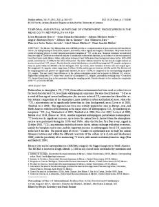
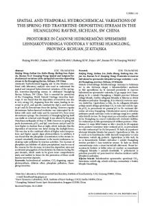
2. Material and methods 2.1. Study sites Field work was carried out in a near-coastal body of water in the Eastern North Sea, 3–18 km off the coast of the barrier island Fanø on the Danish west coast and in the Horsens Fjord, a sheltered fjord system at the east coast of the Jutland peninsula (Fig. 1,2). The North Sea (NS) study site (Fig. 1) is micro-tidal with a semi-diurnal, tidal range of 1.5–1.8 m. Along the easternmost edge of the study area, the water depth is around 4 m
Fig. 1. The study site in the North Sea, off the west coast of the barrier island Fanø. The area hatched with horizontal lines was covered on 14 June, while the area hatched with vertical lines was covered on 11 September. Dots show sampling stations (see also Fig. 3).
Fig. 2. The study area in the Horsens Fjord on the east coast of the Jutland peninsula. The areas delimited by the three shades of grey (from light to dark) indicate the areas investigated at 15 June, 6 September, and 13 June, respectively (see also Fig. 4).
O.A. Mikkelsen / Oceanologica Acta 25 (2002) 39–49
41
Fig. 3. The variation in June and September at the North Sea study site of the temperature (T), total suspended matter concentration (TSM), median beam attenuation coefficient (c50), median particle size (D50), median projected surface area (PSA50), median effective density (∆ρ50), median settling velocity (W50), median vertical flux (Qf50), and chl a. Darker colours show higher values.
at low tide and along the westernmost edge about 16 m. The easternmost edge of the area runs parallel to the shore of the barrier island Fanø, at a distance of 2 km off the shore. The study area lies more or less between two tidal inlets connecting the Wadden Sea with the North Sea: to the north the tidal inlet Grådyb, and to the south the tidal inlet Knudedyb. The area is very exposed to winds from westerly directions and is only in a relatively sheltered position when the wind is from the east. The major resuspension agent is wave activity related to windy periods. Waters in the area are generally well mixed. The NS site can furthermore be considered a transition zone between the Wadden sea area
and the North Sea per se, and is generally not well investigated, compared to these two areas. The Horsens Fjord (HF) (Fig. 2) is also micro-tidal, but with a tidal range of ca. 0.6 m. In general, noticeable water fluctuations in the HF are due to meteorological conditions, not the regular astronomical tide. A halocline with a salinity difference of up to 4–5 is usually present in most of the fjord. For winds from west, north or south, the fetch is only a few kilometres. Only for winds from the east is there a significant wave activity, causing resuspension of bottom sediments and mixing of the stratified water column. Mud or sandy mud constitutes the bottom sediments.
42
O.A. Mikkelsen / Oceanologica Acta 25 (2002) 39–49
median diameter was derived from each PSS. For each station the processed data were grouped into one min intervals, i.e. 36 data sets min–1. Finally, median values for diameter (D50), VC (VC50), and c (c50), were found for each one min interval. Water sampling – Water samples were taken with a 2 L water sampler at the same depth and time as the LISST measurements. TSM was determined by filtering the water samples through pre-filtered, pre-weighed Millipore filters type HA (nominal retention diameter 0.45 µm). The filters were flushed three times with de-ionized water (in order to remove excess salt) and oven dried for 1.5 h at 65 °C. Subsequently the filters were allowed to adjust to room temperature for 0.5 h and weighed with an accuracy of ± 0.1 mg. Pre-weighed blanks followed the same procedure in order to determine whether or not the filters themselves gained or lost weight during the filtration work. Chl a was determined by HPLC from water samples filtered on Whatman GF/F filters. CTD measurements – In the HF a CTD probe (SeaBird SBE 25) was used for obtaining information regarding thermo- and haloclines, while a Kent Temperature Salinity Bridge type MC5 was used in the North Sea. Fig. 4. Examples of CTD measurements of temperature, salinity and normalised turbidity from the Horsens Fjord. Turbidity is normalised to the lowest measured level of turbidity on the three dates. The measurements were all carried out at a station in the middle of the area covered on all three field work dates (cf. Fig. 2).
2.2. Methods 2.2.1. Sampling scheme Particle measurements – Fieldwork was carried out during five days in 1999 at a number of stations. In the NS on 14 June (10 stations) and 11 September (17 stations) and in the HF on 13 June (7 stations), 15 June (11 stations) and 6 September (8 stations). At each station, the particle size spectrum (PSS), the volume concentration (VC), the beam attenuation coefficient (c) and the water temperature was measured in situ one meter below the surface (mbs). Measurements were carried out using an LISST-100 type C laser diffraction particle sizer (Agrawal and Pottsmith, 2000), measuring particle volume in 32 logarithmically spaced size classes in the range 2.5–500 µm. Raw data were sampled at 4 Hz, whereupon average values for five measurements were computed and recorded on the on-board data logger. All stored raw data were thus averaged over a period of 1.25 s. Upon retrieval of the instrument, the raw data were off-loaded and analysed by means of the LISST data processing programme version 3.22, thus yielding the particle size spectrum (PSS), volume concentration (VC), beam attenuation coefficient (c) and the temperature (for details, cf. Agrawal and Pottsmith, 2000). Note that due to the short time it took for the LISST to write data to the data logger, there is a 1.67 s period, not 1.25 s, between each data set consisting of a PSS, VC, c, and temperature. The
2.2.2. Weather conditions On all fieldwork days the weather was much alike. The wind was light, and wave heights were below 0.1–0.5 m at the NS site (lowest in June) and below 0.1–0.2 m in the HF. However, the weather had been quite different in the weeks preceding the June and September study periods. In June, a prolonged period of calm and quiet weather with wave heights generally below 0.4 m persisted in the week up to the 13–15 June. Contrary, in the week before 6–11 September a prolonged period with strong westerly winds and wave heights up to 2 m (in the NS) persisted. Therefore, with respect to wind- and wave-induced energy in the water column, the conditions in the NS were much different from June to September whereas in the HF they were more or less the same, due to the limited fetch in the HF. In the NS, fieldwork on 14 June began 1.5 h after low water and had duration of 5.5 h. On 11 September, fieldwork began 45 min before low water and had duration of 4.25 h. Thus, at the NS site, fieldwork was carried out mainly in the flood period on both study dates. In the HF, fieldwork began less than 2 h before high water and had duration of 6–8 h at all study dates. Therefore, at all study dates in the HF fieldwork were mainly carried out in the ebbing period. 2.2.3. Calculations From the measurements of TSM and VC50, the median effective density, ∆ρ50 and the median settling velocity, W50 of the suspended particles was calculated using equations 1–2 (cf. Mikkelsen and Pejrup 2000, 2001): Dq50 ≈ TSM VC50
(1)
O.A. Mikkelsen / Oceanologica Acta 25 (2002) 39–49
43
Table 1 Area-averaged median values of the investigated parameters, together with their range of variation Date Parameter
The NS, 14 Jun 99
The NS, 11 Sep 99
The HF, 13 Jun 99
The HF, 15 Jun 99
The HF, 6 Sep 99
16.1 15.1–17.0 1.7 1.2–2.1 1.73 1.13–2.20 322 221–425 14.3 9.2–18.4 52 33–90 2.57 1.54–3.94 366 247–700 11.4 6.3–18.6 48.7 10 2.37
18.1 17.8–18.5 2.8 2.0–5.5 1.85 1.11–3.85 117 21–173 16.5 8.6–36.6 98 72–178 0.74 0.03–1.60 171 11–309 5.1 2.3–8.9 67.5 17 2.67
15.7 14.8–16.6 2.2 1.7–2.3 4.42 3.08–5.42 142 95–282 37.4 25.9–47.7 31 22–38 0.32 0.14–0.98 60 25–186 – 1.1–2.2 5.5 7 0.34
15.9 15.0–16.6 2.0 1.4–3.4 3.15 2.24–3.89 164 97–251 26.2 17.9–33.1 38 19–103 0.48 0.23–1.34 90 37–334 1.7 0.8–3.1 9.6 11 0.19
18.4 17.7–18.9 2.7 1.8–3.6 3.48 2.83–5.34 23 17–31 26.7 17.0–44.9 130 107–174 0.03 0.02–0.10 8 4–17 7.2 4.1–14.6 4 8 2.47
T (°C) TSM (mg l–1) c50 (m–1) D50 ( µm) PSA50 (×10–4 m2 l–1) ∆ρ50 (kg m–3) W50 (mm s–1) Qf50 (g m–2 d–1) Chl a ( µg l–1) Area covered (km2) No. of stations Df
T, temperature; TSM, total suspended matter concentration; c50, median beam attenuation coefficient; D50, median particle (aggregate) diameter; PSA50, median projected surface area; ∆ρ50, median effective density; W50, median settling velocity; Qf50, median vertical flux; Df, the fractal dimension of the suspended aggregates; chl a, chlorophyll a concentration.
and D 50 ⋅ Dq50 ⋅ g 18 ⋅ g 2
W50 =
(2)
Equation 2 is Stokes’s Law, where g is gravitational acceleration and g is water viscosity. It should be noted that the W50 computed from (2) may not necessarily be the actual W50, rather the potential W50. The actual W50 could be lower than the potential W50, for example due to turbulence in the water column. Also, it must be recognised that Stokes’s Law should only be used for values of Reynold’s number (Re) < 1. However, it was shown by Sternberg et al. (1999) that inclusion of large aggregates (diameter up to 760 µm) with Re > 1 made no apparent change to their observed relationship between aggregate settling velocity and diameter. In this study, the largest D50 was found to 425 µm (cf. Table 1), suggesting that the use of Stokes’s Law for computation of W50 is suitable. The projected surface area (Bale et al., 1994) of the suspended particles is given according to equation 3 (for details, cf. Mikkelsen, 2001): PSA50 =
32
兺1.5 ⋅ i=1
VCi xI
(3)
where xi is the midpoint of size class i and VCi is the volume concentration in size class i. Again, a PSA was calculated for each size spectrum, and the median value (PSA50) derived for each data set. The PSA can be considered a proxy for remotely sensed water leaving reflectance (Bale et al., 1994; Mikkelsen, 2001). Therefore, it is important to
gain knowledge regarding the potential variation in this parameter. Finally, a potential vertical median flux, Qf50, of the suspended matter can be computed according to equation 4: Qf50 = W50 ⋅ TSM
(4)
3. Results and discussion The spatial and temporal variation of the parameters temperature (°C), TSM (mg l–1), c50 (m–1), D50 (µm), PSA50 (m2 l–1), ∆ρ50 (kg m–3), W50 (mm s–1), Qf50 (g m–2 d–1), and chl a (µg l–1) was mapped for the NS site (Fig. 3a, r) and for the HF (Fig. 5a, z). The median values used for plotting Fig. 3 and 5 are from the same minute where water sampling took place. For each area, the nine parameters were weighted over the entire area in order to find a mean value for each parameter. These are summarized in Table 1. Note that on 13 Jun, the spatial coverage of the chl a sampling was less adequate than for the other parameters, hence it is not mapped for this date in Fig. 5. First, the seasonal variation within each of the study areas is considered. Second, the variation between the NS site and the HF in June and September, respectively, is considered. 3.1. Variation at the NS site From Table 1 and Fig. 3a, b, the water temperature at the NS study site is seen to have risen by approximately 2 °C from June to September. Table 1 and Fig. 3c, d demonstrate
44
O.A. Mikkelsen / Oceanologica Acta 25 (2002) 39–49
Fig. 5. The variation in June and September in the Horsens Fjord of the temperature (T), total suspended matter concentration (TSM), median beam attenuation coefficient (c50), median particle size (D50), median projected surface area (PSA50), median effective density (∆ρ50), median settling velocity (W50), median vertical flux (Qf50), and chl a. Darker colours show higher values.
O.A. Mikkelsen / Oceanologica Acta 25 (2002) 39–49
that TSM has almost doubled; from 1.7 to 2.8 mg l–1 on average, probably related to the windy conditions prior to the September field work. In June there is an increase in TSM when going towards the northwest, while in September there is no clear trend in the distribution of TSM. However, c50 (Fig. 3e, f) is almost constant (∼1.8 m–1) for the two dates. Also the spatial variation in c50 differs from that of TSM: in June, c50 almost doubles towards the west, while in September it is quite constant (∼1.6–1.9 m–1) over a large part of the area. The constant value for c50 is due to the fact that PSA50 is almost constant (Table 1, Fig. 3 i, j). c50 is, in reality, dependent on the PSA50 and will only vary linearly with mass concentration if the in situ particle size and density are constant (Mikkelsen, 2001). The constant value for c thus demonstrates that a change in the in situ size and/or density of the suspended matter has occurred (cf. Mikkelsen, 2001). This is confirmed when considering the change in D50 and ∆ρ50 between the two dates: D50 is reduced to approximately a third between June and September, while ∆ρ50 has almost doubled (Table 1). D50 is quite constant in June, varying approximately a factor of two throughout the area, increasing towards the south west (Fig. 3 g). However, in September D50 varies more than a factor of eight, with a minimum in the northern part and increasing towards the east and west (Fig. 3h). W50 is seen to be almost four times higher in June than September (Fig. 3m, n, Table 1), due to the larger value for D50 in June. There is a slight tendency for W50 to increase towards the west in June, whereas the same pattern as for D50 is observed in September. Also, due to the larger variation in D50 in September than in June, W50 varies more in September. As Qf50 is mainly related to W50, and to a lesser degree TSM, the temporal and spatial variation in Qf50 resembles that of W50 (Fig. 3o, p). Finally, chl a is seen to be quite uniformly distributed in June (Fig. 3q), whereas in September chl a decreases from the centre of the area towards the west and east (Fig. 3 r). Chl a is almost halved from June to September (Table 1). 3.2. Variation in the HF First, a CTD profile obtained in the centre of the area covered at all three study dates is considered (Fig. 4). The thermo- and halocline mentioned above is clearly seen. The maximum temperature difference on the three dates is 5 °C (15 Jun 1999) and the maximum salinity difference is 4.1 (13 Jun 1999). The turbidity measurements reveal that by September turbidity had increased by up to a factor of 2, compared to June. On 15 June, a pronounced increase in turbidity appears close to the bottom. Current measurements were carried out in the fjord on several occasions during an earlier field campaign. These measurements showed that the current velocity 100 cm above the bottom, u100, rarely exceeded 0.05–0.10 m s–1. Such low values of u100 are usually not capable of creating a shear stress strong enough to resuspend sediment. This is espe-
45
cially so in an environment where the bottom sediment is composed mainly of mud. Andersen (1999) showed that for mudflats in the Danish Wadden Sea the regular current with a maximum mean velocity of 0.15–0.20 m s–1 was not capable of resuspending sediment. Only during windy events could the shear stress created by wind-induced waves cause resuspension. TSM is quite constant around 2 mg l–1 on 13 and 15 June, but with a larger variation on 15 June (Table 1). There is a tendency for increasing TSM towards the head of the fjord on 13 June, but this is less clear on 15 June (Fig. 5d, e). c50 has decreased 30% from 13 June to 15 June (Table 1), which is consistent with a decrease in PSA50, related to a slight increase in D50 (Table 1 and Fig. 5g, h). ∆ρ50, W50, and Qf50 for 13 and 15 June are all comparable in magnitude (Table 1). With respect to the spatial variation on 13 and 15 June, it is seen that c50 and PSA50 decrease towards the northern side of the fjord on both dates (Fig. 5g, h, 5m, n). ∆ρ50 is almost constant throughout the fjord on 13 June (Fig. 5p), whereas there is a tendency to an increase towards the west on 15 June (Fig. 5q). W50 and Qf50 increase towards the north side of the fjord on 13 June, but on 15 June there is a slight susceptibility to an increase towards the west (Fig. 5s, t, 5v, w), coincident with the spatial variation in D50 and ∆ρ50. Chl a clearly increases towards the head of the fjord (west) on 15 June (Fig. 5y). Chl a concentrations on 13 and 15 June are of similar magnitude (Table 1). In September, TSM has increased (Table 1). c50 though, is almost equal to the 15 June values, as is PSA50. This is related to a drastic increase in ∆ρ50 from June to September, which combined with a concurrent decrease in D50 serves to keep PSA50 constant. Compared to the values of 15 June, W50 and Qf50 has been reduced by approximately 90%, due to the decrease in D50. TSM, C50, PSA50 and ∆ρ50 now all increase towards the west (Fig. 5f, i, o, r), while no clear tendency exist for D50, W50 or Qf50 (Fig. 5l, u, x). Chl a has increased by more than a factor of three from June to September, with a tendency to a minimum (∼5.5 µg l–1) in the centre of the September study area, and increasing towards the west and east. This is in accordance with observations from fjords nearby, where algae blooms where abundant in September of 1999. The increase in TSM could be related to the increase in chl a, as resuspension of bottom sediments is not very likely to have occurred (cf. discussion above). So, over a short (order of a few days) time scale, and provided that the weather conditions are alike, there seems to be indications that the magnitude of the investigated parameters in the HF does not change to any large degree (Table 1). However, their spatial distribution may well have changed, as demonstrated on Fig. 5d, e, 5j, k, 5p, q, 5v, w. 3.3. Variation between the NS and HF in June From Fig. 3 and 5 and Table 1, it appears that TSM is slightly lower in the NS than in the HF (∼20%). However,
46
O.A. Mikkelsen / Oceanologica Acta 25 (2002) 39–49
c50 is 45–60% lower in the NS than in the HF. As before, this is related to the difference in PSA50 between the two areas. The reason for the much smaller value for PSA50 in the NS is the larger aggregates there, D50 at the NS site being more than a factor of two larger than in the HF. The reason for this is not clear, but it could be related to different algae species and/or algae concentrations at the two dates. From the difference in ∆ρ50 it is seen that the aggregates in the NS are more tightly packed, this could indicate a larger proportion of mineral grains in the NS aggregates. Finally, as W50 is computed from the D50, these values are also larger for the NS than for the HF, between a factor of 4.4 and 7 compared to the HF. Likewise, Qf50 is a factor of 3.7 to 5 larger in the NS. Hence, there seems to be larger potential for mass settling at the NS site than in the HF. However, it must be remembered that the Qf50 is a potential flux only. A large part of the suspended matter in the water column at the study date could have been resuspended matter from within the area, hence giving a false impression of the flux. Chl a is almost a factor of five higher at the NS study site than in the HF. This could be related to advection of Wadden Sea water, which is known to have a high concentration of chl a due to favourable conditions of growth in the Wadden Sea area. 3.4. Variation between the NS and HF in September From Fig. 3 and 5 and Table 1, it is seen that values for TSM are now the same in the two areas, though the range of variation is slightly larger at the NS site than in the HF. c50 is still higher in the HF than in the NS. As for June, this is related to the difference in PSA50, controlled by the difference in D50 and ∆ρ50. The aggregates in the HF are now the more tightly packed, indicating inclusion of mineral grains (perhaps due to resuspension) and/or restructuring of the aggregates due to shear. Most notable is the difference in W50 and Qf50. Compared to June, values have decreased in both areas, but most dramatically in the HF. As for June, there seems to be larger potential for mass settling at the NS site than in the HF. Chl a is now slightly higher in the HF than at the NS site (due to the bloom in HF), compared to the situation in June. 3.5. Overall variation The increase in TSM and the concurrent decrease in D50 and W50 in both areas from June to September could be related to the different meteorological conditions. The windy period in September could easily have caused resus pension of bottom sediments and aggregate break-up, especially at the NS site. As the HF is much more sheltered from the westerly winds, resuspension is probably not the cause for the observed changes in TSM, D50 and W50. Mikkelsen and Pejrup (2001) derived the fractal dimension (Df) for aggregates at the NS and the HF sites in June and September. An increase in the fractal dimension can
occur if the aggregate is restructured to a more compact one, for example due to shear (Kranenburg, 1994; Risovic´ , 1998). Df can be derived from a log-log plot of aggregate effective density vs. aggregate size (cf. van der Lee, 2000). Mikkelsen and Pejrup (2001) used samples from throughout the water column (not only from 1 mbs, as in this study) for their estimates of Df. They reported that Df in the HF was the same in June and September (∼2.3), whereas it increased from 2.1 in June to 2.7 in September at the NS site. Therefore, Mikkelsen and Pejrup (2001) suggested that the reason for the increase in the Df at the NS site was due to the fact that this area was more exposed than the HF. Thus, the stable value for the fractal dimension in the HF suggested that no restructuring had taken place in the HF. In this study, Df was derived for all five study dates, but only for samples taken at 1 mbs (Table 1). It appears that when using the samples from 1 mbs only, the Df now increases from June to September for both the NS and the HF study sites. It would seem that the values for Df presented here somewhat contradicts the findings of Mikkelsen and Pejrup (2001). However, as the Df values presented here (Table 1) are all related to aggregates at 1 mbs, i.e. the upper part of the water column only, the argument that restructuring has taken place might still be valid. While the HF is well sheltered from westerly winds, some turbulence due to wind stress at the surface is still induced in the upper part of the water column, while the lower layers are largely unaffected. As mentioned earlier, a very windy period persisted in the week before the September field work in both the HF and the NS. In the HF, the westerly wind thus would only induce some turbulence close to the surface, causing aggregates to break up and become restructured into more compact entities, thus increasing Df in September as observed. The wind induced turbulence could thus explain the decrease in D50 in both the HF and at the NS site. However, for the HF another explanation is also possible. The change in D50 in the HF could be related to biological processes, such as increased amounts of biogenic exudates. These exudates cause the particles to aggregate and settle out of the upper water column, leaving finer particles and aggregates behind (Avnimelech et al., 1982; Eisma, 1986; Passow et al., 2001). Some evidence for this was found in the particle size spectra from the upper and lower parts of the water column on the stations investigated in September (Fig. 6). Fig. 6a, b are spectra from 1 mbs at two stations in the HF during the September investigation, while Fig. 6c, d are spectra from 0.5 m above the bottom (mab) at the same stations. D50 for the spectra from 1 mbs is ∼18 µm, while it is 89 µm and 366 µm for the spectra from 0.5 mab. It is evident that the aggregates are much larger at 0.5 mab than at 1 mbs, between a factor of 4 and 20 for the spectra shown here. This could be related to the settling of larger aggregates from the surface due to biologically induced aggregation. It has been suggested (Avnimelech et al., 1982; Mari
O.A. Mikkelsen / Oceanologica Acta 25 (2002) 39–49
47
Fig. 7. Examples of the influence of the presence of particles outside the size range of a laser diffraction instrument (Malvern MasterSizer/E). a) Sediment sample analysed with an optical configuration permitting size analysis in the range 0.5-180 µm, median diameter = 32 µm. b) The same sample analysed with an optical configuration of the laser permitting analysis in the size range 1.2-600 µm, median diameter = 30 µm. It is evident that just a small number of particles outside the size range (in this case about 5%) cause a rising “tail” in the size spectrum. However, the influence of particles outside the size range on the median diameter is limited. Fig. 6. Examples of variation in particle size spectra at two stations in the Horsens Fjord, 6 September. A ,b) size spectra from 1 mbs; c, d) size spectra from 0.5 mab (at the same stations as in a, b). Clearly, a change in the size spectra towards the coarser grain-sizes is obvious when moving from the upper part of the water column towards the bed.
and Kiørboe, 1996) that by the end of algae blooms large aggregates tend to form, rapidly removing dying algal cells from the surface waters. Chl a in the HF was more than a factor of three larger in September than in June (Table 1). Therefore, there seems to be some basis for suggesting that biologically induced aggregation in the HF caused aggregation, subsequent settling of the large aggregates into the bottom layer, leaving small particles and aggregates in the upper part of the water column, as demonstrated in Fig. 6a, d. It should be noted that several of the size spectra in Fig. 6a, d exhibit a rising ‘tail’ that is eventually cut off at 500 µm, the upper limit of sizes detected by the LISST-100. In fact, this phenomenon was commonly observed in most of the LISST measurements and it indicates the presence of particles larger than 500 µm (cf. Agrawal and Pottsmith, 2000). The influence of particles outside the measurement range on the D50 is minimal, however. This can be illustrated by Fig. 7, which shows a size analysis of a sediment sample carried out in the laboratory using a Malvern MasterSizer/E laser. The MasterSizer/E can measure particle sizes in three size ranges; 0.1–80 µm, 0.5–180 µm and 1.2–600 µm by changing the optical configuration of the laser. Fig. 7a shows a sediment sample analysed using the 0.5–180 µm configuration. A rising tail at the coarse end of the size spectrum appears. Using the 1.2–600 µm configuration for analysis of the same sample yields the result presented in Fig. 7b. No rising tail appears. It is seen from Fig. 7b that only 4.4% of the entire sample is coarser than
180 µm. More important, the D50 in Fig. 7a, b is, respectively, 31.8 and 30.2 µm. Thus, it may be concluded that the presence of particles outside of the measurement range of laser sizers causes a visible change in the size spectrum, but apparently no significant variation in the D50. The overall variation in W50 (0.03–2.6 mm s–1) is realistic for coastal waters when compared to what is found in the literature. Alldredge and Gotschalk (1989) found individual floc settling velocities between 0.6 and 2.3 mm s–1 for diatom flocs in the Southern California Bight and California Current. Millward et al. (1999) found median settling velocities between 0.001 and 0.2 mm s–1 for suspended matter in the Humber Estuary and the coastal waters off the Holderness, NE-England. Dyer et al. (1996) reports a range in measured values of W50 from 0.0003 to 5 mm s–1 for samples obtained with various kinds of instruments in the Elbe Estuary, Germany. Finally, ten Brinke (1997) reports on W50 varying between 0.6 and 2.4 mm s–1 in the Oosterschelde tidal waters, the Netherlands. Summing up, the values for W50 found in this study (obtained using the method described by Mikkelsen and Pejrup, 2001) are all found to be within the range of values reported in the literature for similar waters. Investigating the relationship between c vs TSM, VC vs TSM and TSM vs PSA (Fig. 8), it is found that there is no significant (P>0.01) correlation. This demonstrates that a large variation in the size and density of the suspended aggregates exists (cf. Mikkelsen, 2001). A highly significant (P