“multiplier-accelerator” model of Hicks and Samuelson (Samuelson 1939).
Aggregate production change in production. Investment. Previous year's GDP.
PAD 724 - PID Control
Page 1
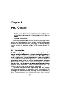
Proportional, Integral, and Derivative Control In this exercise you will formulate a classic (but vastly oversimplified) model of the macroeconomy, which exhibits oscillations reminiscent of business cycles. Following the scheme of A.W. Phillips (see Richardson, Feedback Thought, pp. 136-139), you will then add to the oscillating economic structure a hypothesized government control sector incorporating proportional, integral, and derivative controllers intended to stabilize the economy and hold aggregate production near aggregate demand in the face of economic disturbances. Figure 1 shows the structure of the macroeconomy, a continuous version of the famous “multiplier-accelerator” model of Hicks and Samuelson (Samuelson 1939). Smoothing time for GDP
Accelerator coefficient
Previous year's GDP
Investment Disturbance (Accelerator Loop)
Government spending
Aggregate demand
change in production
Aggregate production
(Multiplier Loop)
Consumption
Production adjustment time Marginal propensity to consume
Comments on the Multiplier-Accelerator Structure The “multiplier” loop is the bottom half of the figure. People consume some fraction of Aggregate Production. That Consumption adds to Aggregate Demand, which is, by the definition of economists, equal to the sum of Consumption, Investment, and Government Spending. Aggregate Production then follows as a SMOOTH of Aggregate Demand, where the smoothing time is given here as the Production Adjustment Time.
PAD 724 - PID Control
Page 2
Astute observers here will see that the multiplier loop is a positive loop wrapped around the negative loop embedded in the smoothing structure. In the positive loop, only a fraction of Aggregate Production feeds around the loop, so the positive loop has less strength (”gain” to engineers) than the negative loop in the smooth. Thus the two-loop “multiplier” structure is actually a goal-seeking structure in which the negative loop dominates. The “accelerator” loop is the structure in the top half of Figure 1. Capital investment in this multiplier-accelerator theory is assumed to be proportional to the trend in production, computed here as Production minus Previous Year’s GNP. The constant of proportionality (the Accelerator Coefficient) is taken here to be 1. Note that Previous Year’s GNP is a SMOOTH3 1 of Production, with a smoothing time (hidden in this figure) of 1 year. The accelerator structure is dominated by its positive loop (since the smoothed Previous Year’s GNP attenuates and lags Production): If Production is rising, then Investment is positive, driving up Aggregate Demand, and causing Production to rise more (other things held constant). If Production is falling, then Investment is negative (depreciation and disinvestment) pulling down Aggregate Demand and causing Production to fall further. In response to a step disturbance [Disturbance = STEP(-50,3)], the multiplier-accelerator model oscillates, as shown below in Figure 2. Note that besides being unstable the system never brings Aggregate Production back up to where it started, which we can take to be Desired Production.
Multiplier-Accelerator 1,000
$/Year
700 400 100 -200 0
4
8
12 Time (Year)
16
20
24
Aggregate demand : mult acc base Aggregate production : mult acc base Investment : mult acc base Consumption : mult acc base Government spending : mult acc base
1
The third order smooth adds a little more instability to the system than a first-order smooth. The oscillations have a slight shorter period and larger amplitude. You can use either SMOOTH or SMOOTH3, as you wish.
PAD 724 - PID Control
Page 3
Figure 3 shows this economic model coupled to a control sector striving to set levels of government spending that stabilize the system and match Aggregate Production to Aggregate Demand. Smoothing time for GDP
Accelerator coefficient Wt on I
chng in cum prod gap
Cumulative production gap
Previous year's GDP
Investment
Integral control Disturbance
Desired production
(Accelerator Loop)
Wt on P
Production gap
Proportional control
Government spending
Aggregate demand
change in production
Recent production gap
Derivative control
Production gap trend
Aggregate production
(Multiplier Loop)
Consumption
Wt on D Time to see trend in production gap
Production adjustment time Marginal propensity to consume
Comments on the Proportional, Integral, and Derivative (PID) Controller The control sector computes the gap between Desired Production (a constant 1000) and Aggregate Production (”ghosted” here on the left from the macroeconomic model on the right). The Production Gap equals Desired Production minus Aggregate Production. The three elements of the control system — proportional, integral, and derivative control — are computed from this Production Gap: Proportional control is directly proportional to the Production Gap, with the constant of proportionality here called the “wt on P,” the weight on proportional control. Integral control is proportional to the accumulated Production Gap, computed in a level whose rate is simply the Production Gap. The “wt on I” is the weight on integral control. Derivative control is directly proportional to the trend in the Production Gap. The trend is computed by smoothing the Production Gap to get the Recent Production Gap and computing the trend (slope) as (Production Gap – Recent Production Gap)/(Time for recent gap). The “wt on D” is the weight on derivative control.
PAD 724 - PID Control
Page 4
The Task Formulate the multiplier-accelerator model linked to the PID control system.2 Simulate the model with the weights on the controllers all set to zero. Duplicate the simulation shown in Figure 2. Then activate the proportional controller, by setting the weight on proportional control to, say, 0.2. What do you observe about the oscillations and the gap between Desired Production and Aggregate Production? Then activate both the proportional controller and the integral controller, by setting their weights to, say, 0.2. What do you observe about the oscillations and the gap between Desired Production and Aggregate Production? Then activate all three controllers. What do you observe about the oscillations and the gap between Desired Production and Aggregate Production? Experiment (as time permits) with other weights on the PID control terms (they need not be equal) and other combinations of control terms. What do you observe about the oscillations and the gap between Desired Production and Aggregate Production? Describe briefly the actions of each of the PID control terms on government spending. [Suggestion: Simulate with the weights each set to 0.2. Draw a causal strip graph for Government Spending and use it to describe what each of the P, I, and D terms are contributing to Government Spending over time.] What would government actually be doing with government spending if it were applying these control efforts? What actors in the system would try to do these things?
2 Technical notes: Set all time constants to 1. Set the Marginal Propensity to Consume to 0.8 (Americans consume
more like 0.94, but let’s be kind) and the Accelerator Coefficient to 1. Set Government Spending equal to 200 plus the sum of the three PID controller terms — government spending will move away from 200 as dictated by the PID control efforts. The initial value of Aggregate Production is computed to put the system into equilibrium (note that Investment is zero in equilibrium, since Production is neither rising nor falling) — you can compute it yourself or read it off the graph. I used DT=.0625 and set the SAVPER to 0.25.