Exercise 1: Getting started with GIS. To get familiar about spatial and surface
analysis functions in SAVGIS. At the end of the exercise, users must be familiar
with ...
Geographic Information System and its Application in Hydro-Meteorology – Exercises using SavGIS Jothiganesh Shanmugasundaram Decision Support Tool Development Specialist COPY DATABASE FOLDER “BHUTAN” in to “SAVBASE” FOLDER. Open Savateca and click Register and define Bhutan folder and click ok. Then only you will be able to work with the database. Exercise 1: Getting started with GIS To get familiar about spatial and surface analysis functions in SAVGIS. At the end of the exercise, users must be familiar with displaying relations, overlaying layers, attribute classification, spatial queries and making map layouts. A. Display relations using Map explorer in SAVANE •
• •
•
Savane �Base�Bhutan� Click “Map Explorer” �Select the relation “Country, District, Sub district” under “objects from database” (Double click the relation or single click the relation and click the Draw Icon) to display in the frame. Click “Map Explorer” �Select the relation “Rainfall Station” under “objects from database” (Double click ) Click “Map Explorer” �Select the relation “SRTMElevation90m” under “objects from database” (Double click) �Select attribute “Altitude” under mosaic �Enable Color gradation and click “>>” � Click “Auto” �Click “Colors” and choose �Click Apply�Click Ok and click Display all tab in Map Explorer. Click “properties” tab and edit the properties of each layer to display in different colour, symbol properties
Figure 1: Administrative boundaries and Topography Map of Bhutan
• • • •
Click “Frame” �Select “Legend” �Edit legend properties �Pencil icon will appear, left click inside the frame to place the legend. Click Text Editor Icon “A” , Type text and left click in the frame to place the text. Click “Frame” �Click North Arrow & Graphical Scale �Pencil icon will appear, left click inside the frame to place the north arrow and graphical scale. Select “Frame” �Right click and select “Screen Capture” �Define the directory and file name.
B. Import Population data from Excel file •
Select “Frame” � Import attributes �From an Excel file �Define the directory for the population file “District_population” in Data folder � Select relation “District” and select the attribute “Name” �Next �select the tables under “Tables to integrate with” and click “Name” under the column “Join with” � Finish
C. Compute Population density by district •
Click “Compute” � select “Area” menu �select the relation “District” � Select unit “square kilometer” and enable “Maximum accuracy” and click “ok”. It will create a new attribute called “Area” in the relation District.
•
Click “Compute” � select “Numerical Calculations” menu � “Formula” � Select the relation “District”. Type the formula “v[population]/v[Area]”� then click next � Give name for the new attribute “Density” and click “Finish”
D. •
Manual classification of Population attribute Click “Class” � select “user delimited intervals” menu � Select the relation “District” �Select attribute “Density” � then define the interval and give the name “DensityRC”
Figure 2: Screen capture of Reclassifying classes using “User Delimited interval function”
•
• • • •
Click “Map Explorer” �Select the relation “District” under “objects to display” �”Properties” �Zone � “Fill zones according to one attribute” � Select “DensityRC” � click >> next to the colors and patterns �Define colour for each class and Click OK. Click “Frame” �Select “Legend” �Edit legend properties �Pencil icon will appear, left click inside the frame to place the legend. Click Text Editor Icon “A”, Type text and left click in the frame to place the text. Click “Frame” �Click North Arrow & Graphical Scale �Pencil icon will appear, left click inside the frame to place the north arrow and graphical scale. Select “Frame” �Right click and select “Screen Capture” �Define the directory and file name.
Figure 3: Population Density Map of Bhutan by district Question: Where can you use this method? Give two examples or situation where it is more applicable?
Exercise 2: Surface Analysis of TRMM rainfall data To get familiar about handling TRMM rainfall grid datasets in GIS. Description of the Exercise A. Three hourly or Daily or Monthly data in ASCII format is easily available in the following link http://disc2.nascom.nasa.gov/Giovanni/tovas/TRMM_V6.3B42.2.shtml
Users can define their geographical extent and download the data for required period by clicking Ascii format in the webpage. New webpage will pop-up with ascii data set. Save the popup web page as text file to your computer. Open the text file and delete first five lines, so that the file should have Latitude, Longitude, AccRain at first line and data follows. Import these monthly rainfall data as column in Excel file and have one excel file for one year to integrate into GIS.
Data Sample Example file is available in the following path \Data\TRMM_Obs\TRMM_24May2009.txt Creating a Relation and Attribute •
Open SAVATECA � Click Base � Select Bhutan and Click OK� Click the menu Scheme � Select Relations under Scheme �Click the Create Button in the Relation Manager window � Assign the name of the relation “TRMM24May09” and Choose the Type “Point” and Click OK
•
Click the menu Scheme � Select Attributes � Select the relation TRMM24May09 � Click Add button � Assign the name of the attribute “Rainfall” and Choose the Type Numeric �Click >> and Click OK Modify External View
•
Click External views �Click Modify �Choose “view” �Click OK � Select the relation “TRMM24May09” and click “Add relations” or Double click the relation under “TRMM24May09”, it will appear under “Visible relations” Data Integration from Text file
•
Integrate � Location-based objects � Points with id only (ASCII format) � Points integration window will popup, Select the relation name (TRMM24May09) where you want to integrate � Select the attribute (Rainfall) �Click Next �Define the path where the ASCII file is stored “\Data\TRMM_Obs\TRMM_24May2009.txt” and select the file �Select the document under “Available documents” � Select the delimiter type ( for our exercise) �if first row in data is description, then enable the Field headers �Click Next �Assign the Longitude (2) and latitude (1) field no. and click Next �Select the attribute “Rainfall” and assign the field no. (4) in “field in external file” �Click >> �Click Test �Click Finish. Data Visualization in SAVANE
•
Open Savane → Base → Bhutan →Babel → Interpolation → Select the relation TRMM21May09 → Define the attribute which you want to interpolate (Rainfall) → Define the name for the new attribute “RF24May or any” and then Click Next → Choose the interpolation method “Barycentric over Neighbors – Two Steps” to make the process fast → Click Next and Finish the process.
•
Class → User delimited interval → Select the relation RASTER and attribute RF24May (interpolated attribute) → Type the numbers from lower limit to upper limit one by one 1,10,25,50, 100,200,300 and the give a new name (RF24MayRC) for this attribute and Finish the process.
•
Map Explorer → Double click the layer Raster and select the attribute RF24MayRC to display in the screen → Change the “color gradation” → Place north arrow, scale bar, legends, grid lines, and boundaries.
Figure 4: TRMM Rainfall surface map of Bhutan – 24May2009 Exercise for Practice: Do the same procedures for plotting the rest of the TRMM data file in the following path “\Data\TRMM_Obs\*.May2009.txt” Multiple Data Integration from Excel File User can import five days rainfall data as attributes in a single relation. Import these daily rainfall data files as column in Excel file and have one excel file for one year to integrate into GIS. Step1: Import text files one by one into EXCEL file Lat|Lon|AccRain|Lat|Lon|AccRain|Lat|Lon|AccRain|Lat|Lon|AccRain|Lat|Lon|AccRain Step2: Rename the column names with respective dates Lat|Lon|21May09|Lat|Lon|22May09|Lat|Lon|23May09|Lat|Lon|24May09|Lat|Lon|25May09 Step3: Keep the first Lat|Lon and remove all other Lat|Lon columns in the file Lat|Lon|21May09| 22May09 |23May09| 24May09| 25May09 Step4: Save the Excel file Step5: Savateca →Base →Bhutan →Create a new relation RFTRMM →Add attributes from 21May, 22May, 23May, 24May, 25May (5 attributes). Integrate →Location based objects →Points with id and other attributes (Excel format) →Browse and select your excel file and define Lat. (1) Lon(2) position and projection details(Geographic) →Define attribute position in Excel file, for example 21May09 as 3, 22May09 as 4, 23May09 as 5, 24May09 as 6, 25May09 as 7 → Click Finish to end the process → External views →Modify → Double click the relation RFTRMM to make it visible. Step6: Open Savane → Interpolate and make Map layout using SAVANE as explained for previous exercise.
Exercise 3: Surface Observatory rainfall data To get familiar about handling observatory rainfall datasets in GIS. Integrate New Data Data can be separated with columns in Excel file “Name Lat Column1: Column2: Column3: Column4:
Lon
May2009”
Name of station Latitude Longitude May2009
Savateca →Base →Bhutan →Create a new relation “RFOBS” →Add attributes Name (Nominal), May2009 (Numeric). Integrate →Location based objects →Points with id and other attributes (Excel format) →Browse and select your excel file and define Lat. (2) Lon(3) position and projection details(Geographic) →Define attribute position in Excel file, for example Name as 1, May09 as 4, → Click Finish to end the process → External views →Modify → Double click the relation RFTRMM to make it visible. Open Savane → Interpolate and make Map layout using SAVANE as explained for previous exercise. Adding Temporal Data to Existing Station in GIS database (PERMANENT) Create one Excel file and add columns for every month or day or year and save it. “Name
June2009
July2009
Aug2009
Sep2009
etc…”
Savateca →Base →Bhutan → Values using a Join →Excel Sheet →Select the relation “RFOBS” and attribute “Name” →Define the path of the Excel file which you saved →Select the sheet under “Select table to integrate” → select the key attribute “Name” under “Attribute to integrate with” → Browse and select your excel file and define attribute position in Excel file, for example June2009 as 2, July2009 as 3, Aug2009 as 4 etc.,→ Click Finish to end the process → External views →Modify → Double click the relation RFOBS and select the newly created attributes to make it visible. Adding Temporal Data to Existing Station in GIS database (TEMPORARY) Create one Excel file and add columns for every month or day or year and save it. “Name
June2009
July2009
Aug2009
Sep2009
etc…”
Savane →Import attributes→From an Excel file → Define the path of the Excel file which you saved and click Open → Select the relation “RFOBS” and attribute “Name” → Select the sheet under “Select table to integrate” → select the key attribute “Name” under “Attribute to integrate with” → Click Finish to end the process
Data Visualization in SAVANE •
Open Savane → Base → Bhutan →Babel → Interpolation → Select the relation RFOBS → Define the attribute which you want to interpolate (May2009) → Define the name for the new attribute “May09obs or any” and then Click Next → Choose the interpolation method “Barycentric over Neighbors – Two Steps” to make the process fast → Click Next and Finish the process.
•
Class → User delimited interval → Select the relation RASTER and attribute May09Obs(interpolated attribute) → Type the numbers from lower limit to upper limit one by one 1,10,25,50, 100,200,300 and the give a new name (May09obsRC) for this attribute and Finish the process.
•
Map Explorer → Double click the layer Raster and select the attribute 21day1fcstRC to display in the screen → Change the “color gradation” → Display District boundaries with names, Place north arrow, scale bar, legends, grid lines, and boundaries.
Exercise 4: RIMES WRF Forecast Plot in GIS To get familiar about handling WRF forecast data in GIS. All Grid data can be imported into a GIS database if it has geographic coordinates. FORTRAN Program enables us to write the WRF model output data into GIS compatible format. Data Sample Example file is available in the following path \Data\RIMES_WRF\wrfrain21may09.txt
Column Column Column Column Column
1: 2: 3: 4: 5:
Longitude Latitude Rainday1forecast Rainday2forecast Rainday3forecast
Initial condition for the file wrfrain21may09 is 21May2009 12UTC. Following are the day1, day2 and day3 forecasts. • • •
Rainday1forecast (22May2009 00UTC to 23May2009 00UTC) Rainday2forecast (23May2009 00UTC to 24May2009 00UTC) Rainday3forecast (24May2009 00UTC to 25May2009 00UTC)
Creating a Relation and Attribute •
Open SAVATECA � Click Base � Select Bhutan and Click OK� Click the menu Scheme � Select Relations under Scheme �Click the Create Button in the Relation Manager window � Assign the name of the relation “wrfrain21may09” and Choose the Type “Point” and Click OK
•
Click the menu Scheme � Select Attributes � Select the relation wrfrain21may09 � Click Add button � Assign the name of the attribute “Day1fcst, Day2fcst, Day3fcst” and Choose the Type Numeric �Click >> and Click OK Modify External View
•
Click External views �Click Modify �Choose “view” �Click OK � Select the relation “wrfrain21may09” and click “Add relations” or Double click the relation under “wrfrain21may09”, it will appear under “Visible relations” Data Integration from Text file
•
Integrate � Location-based objects � Points with id only (ASCII format) � Points integration window will popup, Select the relation name (wrfrain21may09) where you want to integrate � Select the attribute (Rainfall) �Click Next �Define the path where the ASCII file is stored “\Data\RIMES_WRF\wrfrain21may09.txt” and select the file �Select the document under “Available documents” � Select the delimiter type ( for our exercise) �if first row in data is description, then enable the Field headers �Click Next �Assign the Longitude (1) and latitude (2) field no. and click Next �Select the attribute “Day1fcst” and assign the field no. (4) in “field in external file” and similarly for the attribute “Day2fcst” – field no(5) and for the attribute “Day3fcst” –field no. (6) �Click >> �Click Test �Click Finish. Data Visualization in SAVANE
•
Open Savane → Base → Bhutan →Babel → Interpolation → Select the relation wrfrain21may09 → Define the attribute which you want to interpolate (Day1fcst) → Define the name for the new attribute “21day1fcst or any” and then Click Next → Choose the interpolation method “Barycentric over Neighbors – Two Steps” to make the process fast → Click Next and Finish the process.
•
Class → User delimited interval → Select the relation RASTER and attribute RF24May (interpolated attribute) → Type the numbers from lower limit to upper limit one by one 1,10,25,50, 100,200,300 and the give a new name (21day1fcstRC) for this attribute and Finish the process.
•
Map Explorer → Double click the layer Raster and select the attribute 21day1fcstRC to display in the screen → Change the “color gradation” → Display District boundaries with names, Place north arrow, scale bar, legends, grid lines, and boundaries.
Figure 5 Map showing RIMES WRF forecast map(25May2009 Day1 fcst) for Bhutan region.
Figure 6: Map showing RIMES WRF forecast map(25May2009 Day2 fcst) for Bhutan region.
Figure 7: Map showing RIMES WRF forecast map (25May2009 Day3 fcst) for Bhutan region. Exercise 5: Exposure Assessment A sample case study is assumed for Bhutan based on Aila Cylone Impact. It is known that Punatsangchu river is flooded during 25May2009. So
Visualizing elements at risk in Flood Hazard prone area •
Open Savane → Base → Bhutan →Mask → Create → Around Objects →Select the relation “Floodriver” → Assign width around objects “2000” m and save as 2kmbuffer . Repeat the same by assigning 5000m and 10000m and save as 5kmbuffer, 10kmbuffer respectively.
•
Mask → Integrate → Select “2kmbuffer” and enable “Zone and assign name “HighHZ”. Repeat the same by selecting “5kmbuffer,10kmbuffer” and save as “MedHZ, LowHZ” respectively
•
Map Explorer → Display relations one by one “Floodriver”, District boundary, HighHZ, MedHZ, LowHZ, PopulationGRUMP” → Edit the properties to display in different colour.
Spatial Queries to know elements at risk in 10km buffer region Query → Restriction →Using a Mask →Select the relation Subdistrict → Click Next →Select the mask “10kmbuffer” →Enable “Select the intersection” → click Finish Query → List Values → Select the relation Subdistrict → Click Next → Select the attribute “Name” → Click Finish Query → Restriction →Using a Mask →Select the relation “PopulationGRUMP” → Click Next →Select the mask “10kmbuffer →Enable “Select the intersection” → click Finish Stat → Explorer → Select the relation “PopulationGRUMP” .Check the Sum value of population in the popup window
Repeat the same for 5kmbuffer and 2km buffer. Tabulate the results Exercise 6: Hydrological Station Location Plot Integrate New Data Data can be separated with columns in Excel file
Column1: Column2: Column3: Column4: Column5:
ID StationNo. StationName Latitude Longitude
Savateca →Base →Bhutan →Create a new relation “Hydrologystation” →Add attributes ID, StationName (Nominal), StationNo (Numeric). Integrate →Location based objects →Points with id and other attributes (Excel format) →Browse and select your excel file and define Lat. (4) Lon(5) position and projection details(Geographic) →Define attribute position in Excel file, for example ID as 1 and station No as 2 and StationName as 3 → Click Finish to end the process → External views →Modify → Double click the relation RFTRMM to make it visible. Adding Temporal Data to Existing Station in GIS database (PERMANENT)
Create one Excel file and add columns for every month or day or year and save it. “ID
StationNo.
StationName
Lat
Lon
Hmax10May09 Hmax11May09 etc.,”
Savateca →Base →Bhutan → Values using a Join →Excel Sheet →Select the relation “Hydrologystation” and attribute “Name” →Define the path of the Excel file which you saved →Select the sheet under “Select table to integrate” → select the key attribute “ID” under “Attribute to integrate with” → define attribute position in Excel file, for example Hmax10May09 as 6, Hmax11May09 as 7 etc.,→ Click Finish to end the process → External views →Modify → Double click the relation Hydrologystation and select the newly created attributes to make it visible. Adding Temporal Data to Existing Station in GIS database (TEMPORARY) Create one Excel file and add columns for every month or day or year and save it. “ID
StationNo.
StationName
Lat
Lon
Hmax10May09 Hmax11May09 etc.,”
Savane →Import attributes→From an Excel file → Define the path of the Excel file which you saved and click Open → Select the relation “Hydrologystation” and attribute “ID” → Select the sheet under “Select table to integrate” → select the key attribute “Name” under “Attribute to integrate with” → Click Finish to end the process