Jan 25, 2015 - MMMMMM YYYY, Volume VV, Code Snippet II. http://www.jstatsoft.org/ ... The R package RegressionFactory provides expander functions for ...
JSS
Journal of Statistical Software
arXiv:1501.06111v1 [stat.CO] 25 Jan 2015
MMMMMM YYYY, Volume VV, Code Snippet II. http://www.jstatsoft.org/
Expander Framework for Generating High-Dimensional GLM Gradient and Hessian from Low-Dimensional Base Distributions: R Package RegressionFactory Alireza S. Mahani
Mansour T.A. Sharabiani
Scientific Computing Group Sentrana Inc.
National Heart and Lung Institute Imperial College London
Abstract The R package RegressionFactory provides expander functions for constructing the high-dimensional gradient vector and Hessian matrix of the log-likelihood function for generalized linear models (GLMs), from the lower-dimensional base-distribution derivatives. The software follows a modular implementation using the chain rule of derivatives. Such modularity offers a clear separation of case-specific components (base distribution functional form and link functions) from common steps (e.g., matrix algebra operations needed for expansion) in calculating log-likelihood derivatives. In doing so, RegressionFactory offers several advantages: 1) It provides a fast and convenient method for constructing log-likelihood and its derivatives by requiring only the low-dimensional, base-distribution derivatives, 2) The accompanying definiteness-invariance theorem allows researchers to reason about the negative-definiteness of the log-likelihood Hessian in the much lowerdimensional space of the base distributions, 3) The factorized, abstract view of regression suggests opportunities to generate novel regression models, and 4) Computational techniques for performance optimization can be developed generically in the abstract framework and be readily applicable across all the specific regression instances. We expect RegressionFactory to facilitate research and development on optimization and sampling techniques for GLM log-likelihoods as well as construction of composite models from GLM lego blocks, such as Hierarchical Bayesian models.
Keywords: negative definiteness, regression, optimization, sampling, monte carlo markov chain, hierarchical bayesian.
2
Regression Expander Functions: R Package RegressionFactory
1. Introduction Generalized Linear Models (GLMs) (McCullagh and Nelder 1989) are one of the most widelyused classes of models in statistical analysis, and their properties have been thoroughly studied and documented (see, for example, Dunteman and Ho (2006)). Model training and prediction for GLMs often involves Maximum-Likelihood estimation (frequentist approaches) or posterior density estimation (Bayesian approaches), both of which require application of optimization or MCMC sampling techniques to the log-likelihood function or some function containing it. Differentiable functions often benefit from optimization/sampling algorithms that utilize the first and/or second derivative of the function (Press 2007). With proper choice of link functions, many GLMs have log-likelihood functions that are not only twicedifferentiable, but also globally-concave (Gilks and Wild 1992), making them ideal candidates for optimization/sampling routines that take advantage of these properties. For example, the most common optimization approach for GLMs is Iterative Reweighted Least Squares (IRLS) (Gentle 2007, Section 6.8.1). IRLS is a disguised form of Newton-Raphson optimization (Wright and Nocedal 1999), which uses both the gradient and Hessian of the function, and relies on global concavity for convergence. When Hessian is too expensive to calculate or lacks definiteness, other optimization techniques such as conjugate gradient (Press 2007, Section 10.6) can be used, which still require the first derivative of the function. Among MCMC sampling algorithms, Adaptive Rejection Sampler (Gilks and Wild 1992) uses the first derivative and requires concavity of the log-density. Stochastic Newton Sampler (Qi and Minka 2002; Mahani, Hasan, Jiang, and Sharabiani 2014), a Metropolis-Hastings sampler using a locally-fitted multivariate Gaussian, uses both first and second derivatives and also requires log-concavity. Other techniques such as Hamiltonian Monte Carlo (HMC) (Neal 2011) use the first derivative of log-density, while their recent adaptations can use second and even third derivative information to adjust the mass matrix to local space geometry (Girolami and Calderhead 2011). Efficient implementation and analysis of GLM derivatives and their properties, therefore, is a key component to our ability to build probabilistic models using the powerful GLM framework. The R package RegressionFactory contributes to computational research and development on GLM-based statistical models by providing an abstract framework for constructing, and reasoning about, GLM-like log-likelihood functions and their derivatives. Its modular implementation can be viewed as code factorization using the chain rule of derivatives (Apostol 1974). It offers a clear separation of generic steps (expander functions) from model-specific steps (base functions). New regression models can be readily implemented by supplying their base function implementation. Since base functions are in the much lower-dimensional space of the underlying probability distribution (often a member of the exponential family with one or two parameters), implementation of their derivatives is much easier than doing so in the high-dimensional space of regression coefficients. A by-product of this code refactoring using the chain rule is an invariance theorem governing the negative definiteness of the loglikelihood Hessian. The theorem allows this property to be studied in the base-distribution space, again a much easier task than doing so in the high-dimensional coefficient space. The modular organization of RegressionFactory also allows for performance optimization techniques to be made available across a broad set of regression models. This is particularly true for optimizations applied to expander functions, but also applies to base functions since they share many concepts and operations across models. RegressionFactory contains a lower-level set of tools compared to the facilities provided by mainstream regression utilities such as
Journal of Statistical Software – Code Snippets
3
the glm command in R, or the package dglm (Dunn and Smyth 2014) for building double (varying-dispersion) GLM models. Therefore, in addition to supporting research on optimization/sampling algorithms for GLMs as well as research on performance optimization for GLM derivative-calculation routines, exposing the log-likelihood derivatives using the modular framework of RegressionFactory allows modelers to construct composite models from GLM lego blocks, including Hierarchical Bayesian models (Gelman and Hill 2006). The rest of the paper is organized as follows. In Section 2, we begin with an overview of GLM models and arrive at our abstract, and expanded, representation of GLM log-likelihoods (2.1). We then apply the chain rule of derviatives to this abstract expression to derive two equivalent sets of factorized equations (compact and explicit forms) for computing log-likelihood gradient and Hessian using their base-function counterparts (2.2). We use the explicit forms of the equations to prove a negative-definiteness invariance theorem for the log-likelihood Hessian (2.3). Section 3 discusses the implementation of the aforementioned factorized code in RegressionFactory using the expander functions (3.1) and the base functions (3.2). In Section 4, we illustrate the use of RegressionFactory using examples from single-parameter and multi-parameter base functions. Finally, Section 5 contains a summary and discussion.
2. Theory In this section we develop the theoretical foundation for RegressionFactory, beginning with an overview of GLM models.
2.1. Overview of GLMs In GLMs, response variable1 y is assumed to be generated from an exponential-family distribution, and its expected value is related to linear predictor xt β via the link function g: g(E(y)) = xt β.
(1)
where x is the vector of covariates and β is the vector of coefficients. For single-parameter distributions, there is often a simple relationship between the distribution parameter and its mean. Combined with Equation 1, this is sufficient to define the distribution in terms of the linear predictor, xt β. For many double-parameter distributions, the distribution can be expressed as yθ − B(θ) fY (y; θ, Φ) = exp{ + C(y, Φ)} (2) Φ where range of y does not depend on θ or Φ. This function can be maximized with respect to θ without knowledge of Φ. Same is true if we have multiple conditionally-independent data points, where log-likelihood takes a summative form. Once θ is found, we can find Φ (dispersion parameter) through maximization or method of moments, as done by glm in R. Generalization to varying-dispersion models is offered in the R package dglm, where both mean and dispersion are assumed to be linear functions of covariates. In dglm estimation is done iteratively by alternating between an ordinary GLM and a dual GLM in which the deviance components of the ordinary GLM appear as responses (Smyth 1989). 1 To simplify notation, we assume that response variable is scalar, but generalization to vector response variables is straightforward.
4
Regression Expander Functions: R Package RegressionFactory
In RegressionFactory, we take a more general approach to GLMs that encompasses the glm and dglm approaches but is more flexible. Our basic assumption is that log-density for each data point can be written as: � log P(y | { xj }j=1,...,J ) = f (< x1 , β 1 >, . . . , < xJ , β J >, y)
(3)
where < a, b > means inner product of vectors a and b. Note that we have absorbed the nonlinearities introduced through one or more link functions into the definition of f . For N conditionally-independent observations y1 , . . . , yN , the log-likelihood as a function of coefficients β j is given by: L(β 1 , . . . , β J ) =
N X
fn (< x1n , β 1 >, . . . , < xJn , β J >),
(4)
n=1
where we have absorbed the dependence of each term on yn into the indexes of the base functions fn (u1 , . . . , uJ ). P With proper choice of nonlinear transformations, we can assume j that the domain of L is R j K , where K j is the dimensionality of β j . This view of GLMs naturally unites single-parameter GLMs such as Binomial (with fixed number of trials) and Poisson, constant-dispersion two-parameter GLMs (e.g. normal and Gamma), varying-dispersion two-parameter GLMs (e.g. heteroscedastic normal regression), and multi-parameter models such as multinomial logit. It can motivate new GLM models such as geometric (see Section 4.3) and exponential, and can even include survival models (see, e.g., BSGW package (Mahani and Sharabiani 2014)). Several examples are discussed in Section 4. Our next stepPis to apply the chain rule of derivatives to Equation 4 to express the highdimensional ( j K j ) derivatives of L in terms of the low-dimensional (J) derivatives of fn ’s. We will see that the resulting expressions offer a natural way for modular implementation of GLM derivatives.
2.2. Application of chain rule First, we define our notation for P representing derivative objects. We concatenate all J coefficient vectors, β j ’s, into a single j K j -dimensional vector, β: β ≡ (β 1,t , . . . , β J,t )t .
(5)
The first derivative of log-likelihood can be written as: G(β) ≡ where (
∂L ∂L ∂L = (( 1 )t , . . . , ( J )t )t , ∂β ∂β ∂β
∂L t ∂L ∂L ) ≡ ( j , . . . , j ). j ∂β ∂β1 ∂βK j
(6)
(7)
For second derivatives we have: H(β) ≡
� � ∂2L ∂2L = , 0 ∂β 2 ∂β j ∂β j j,j 0 =1,...,J
(8)
Journal of Statistical Software – Code Snippets where we have defined H(β) in terms of J 2 matrix blocks: " # ∂L ∂2L 0 0 ≡ ∂β j ∂β j ∂βkj ∂βkj 0 j=1,...,K j ;j 0 =1,...,K j 0
5
(9)
Applying the chain rule to the log-likelihood function of Equation 4, we derive expressions for its first and second derivatives as a function of the derivatives of the base functions f1 , . . . , fN : N
N
X ∂fn X ∂fn ∂L = = xj = Xj,t gj , j ∂uj n ∂β j ∂β n=1 n=1 with gj ≡ (
∂f1 ∂fN t ,..., ), j ∂u ∂uj
(10)
(11)
and Xj ≡ (xj1 , . . . , xjN )t .
(12)
Similarly, for the second derivative we have: N
N
X ∂ 2 fn X ∂ 2 fn ∂2L j j0 j,t jj 0 j 0 h X , = = 0 (xn ⊗ xn ) = X 0 0 j j j j j j ∂u ∂u ∂β ∂β ∂β ∂β n=1 n=1
(13)
0
where hjj is a diagonal matrix of size N with n’th diagonal element defined as: ∂ 2 fn (14) ∂uj ∂uj 0 We refer to the matrix form of the Equations 10 and 13 as ‘compact’ forms, and the explicitsum forms as ‘explicit’ forms. The expander functions in RegressionFactory use the compact form to implement the high-dimensional gradient and Hessian (see Section 3.1), while the definiteness-invariance theorem below utilizes the explicit-sum form of Equation 13. 0
hjj n ≡
2.3. Definiteness invariance of Hessian Theorem 1. If all fn ’s in Equation 4 have negative definite Hessians AND if at least one of J matrices Xj ≡ (xj1 , . . . , xjN )t is full rank, then L(β 1 , . . . , β J ) also has a negative-definite Hessian. Proof. To prove negative-definiteness of H(β) (hereafter P referred to as H for brevity), we seek j t to prove that p Hp is negative for all non-zero p in R j K . We begin by decomposing p into J subvectors of length K j each: p = (p1,t , . . . , pJ,t )t .
(15)
We now have: t
p Hp =
J X
pj,t
j,j 0 =1
=
X
j,t
p
j,j 0
=
∂2L 0 pj j j0 ∂β ∂β
(16)
! X ∂ 2 fn 0 j j0 . (xn ⊗ xn ) pj j ∂uj 0 ∂u n
(17)
X X ∂ 2 fn 0 0 j,t (xjn ⊗ xjn ) pj 0 p j j ∂u ∂u 0 n j,j
(18)
6
Regression Expander Functions: R Package RegressionFactory
If we define a set of new vectors qn as: � qn ≡ p1,t x1n · · ·
� pJ,t xJn ,
(19)
and use hn to denote the J-by-J Hessian of fn : 0
hn ≡ [hjj n ]j,j 0 =1,...,J ,
(20)
X
(21)
we can write: pt Hp =
qtn hn qn .
n
Since all hn ’s are assumed to be negative definite, all qtn hn qn terms must be non-positive. Therefore, pt Hp can be non-negative only if all its terms are zero, which is possible only if all qn ’s are zero vectors. This, in turn, means we must have pj,t xjn = 0, ∀ n, j. In other words, we must have Xj pj = ∅, ∀ j. This means that all Xj ’s have non-singleton nullspaces and therefore cannot be full-rank, which contradicts our assumption. Therefore, pT Hp must be negative. This proves that H is negative definite. Proving negative-definiteness in the low-dimensional space of base functions is often much easier. For single-parameter distributions, we simply have to prove that the second derivative is negative. For two-parameter distributions, and according to Silvester’s criterion (Gilbert 1991), it is sufficient to show that both diagonal elements of the base-distribution Hessian as well as its determinant are negative. Note that negative-definiteness depends not only on the distribution but also on the choice of link function(s). For twice-differentiable functions, negative-definiteness of Hessian and log-concavity are equivalent (Boyd and Vandenberghe 2009). Gilks and Wild (1992) have a list of log-concave distributions and link functions.
3. Implementation RegressionFactory is a direct implementation of compact expressions in Equations 10 and 13. These expressions imply a code refactoring by separating model-specific steps (calculation of 0 gj and hjj ) from generic steps (calculation of linear predictors Xj β j as well as Xj,t gj and 0 0 Xj,t hjj Xj ). This decomposition is captured diagramatically in the system flow diagram of Figure 1.
3.1. Expander functions Current implementation of RegressionFactory contains expander and base functions for oneparameter and two-parameter distributions. This covers the majority of interesting GLM cases, and a few more. A notable exception is multinomial regression models (such as logit and probit) which can have an unspecified number of slots. The package can be extended in the future to accommodate such more general cases.
Single-parameter expander function Below is the source code for regfac.expand.1par:
Journal of Statistical Software – Code Snippets
7
j
input
{X } {b j }
f
output
j
G={G }
jj'
H={{ H }}
{ X j bj }
{u j }
∑n f n
{f n }
{ X j ,t g j }
{{gn }}
{{X j , t h jj ' X j ' }}
{{{hnjj' }}}
j
Base Function (Vectorized)
Expander Function
Figure 1: System flow diagram for RegressionFactory. The expander function is responsible for calculation of log-likelihood and its gradient and Hessian in the high-dimensional space of regression coefficients. It does so by calculating the linear predictors and supplying them to the base function, which is responsible for calculation of log-likelihood and its gradient and Hessian for each data point, in the low-dimensional space of the underlying probability distribution. The expander function converts these low-dimensional objects into the highdimensional forms, using generic matrix-algebra operations. .
8
Regression Expander Functions: R Package RegressionFactory
R> regfac.expand.1par