The expected kernel for missing features is introduced and applied to training a support vector machine. The expected kernel is a measure of the mean similarity ...
EXPECTED KERNEL FOR MISSING FEATURES IN SUPPORT VECTOR MACHINES Hyrum S. Anderson
Maya R. Gupta
Sandia National Laboratories1 Data Analysis and Exploitation Department Albuquerque, NM 87123
University of Washington Department of Electrical Engineering Seattle, WA 98125
ABSTRACT The expected kernel for missing features is introduced and applied to training a support vector machine. The expected kernel is a measure of the mean similarity with respect to the distribution of the missing features. We compare the expected kernel SVM with the robust second-order cone program (SOCP) SVM, which accounts for missing kernel values by estimating the mean and covariance of missing similarities. Further, we extend the SOCP SVM to utilize the expected kernel by deriving the expected kernel variance. Results show that the expected kernel—used with a traditional SVM solver—shows competitive performance on benchmark datasets to the SOCP SVM at a far-reduced computational burden. Index Terms— missing features, support vector machine, kernel, expected kernel 1. INTRODUCTION Data with missing features is a common problem encounted in signal processing, statistics and machine learning. A standard solution is to impute the missing values, for example by replacing the values with the average of all other related data instances, or using k nearest neighbors (k-NN) of each instance to fill in missing values (also called hot deck imputation). Farhangfar et al. recently analyzed the effect of imputing missing features in training data using several standard imputation strategies, and found that classification accuracy of support vector machine (SVM) and k-NN classifiers generally benefit from imputation [1]. In multiple imputation, each missing value is replaced by a list of m > 1 plausible values, producing m plausible alternative versions of the complete data [2]. Classification or regression algorithms can be run independently on each of the m datasets, then averaged Monte-Carlo style to form an output and a variance that reflects missing-data uncertainty. 1 Sandia National Laboratories is a multi-program laboratory managed and operated by Sandia Corporation, a wholly owned subsidiary of Lockheed Martin Corporation, for the U.S. Department of Energy’s National Nuclear Security Administration under contract DE-AC04-94AL85000.
Multiple imputation has been used to compute support vector machines (SVM) kernels to handle missing features [1]. Rather than form a discrete set of multiple imputation candidates, we propose using the expected kernel—the mean similarity value over the distribution of possible candidates— with an SVM. Expected kernels have been used to incorporate uncertainty due to additive and channel noise on test signals [3], and the same formulation has also been termed marginalized kernel and used to marginalize out hidden variables when computing kernels between graphs [4]. Here we show that the expected kernel is an effective and efficient approach to the missing features problem. In related work, Shivaswamy et al. introduced a generalization of the SVM so that the margin-maximization takes into account the uncertainty due to missing features or noise [5]. The resulting second-order cone program (SOCP) SVM is discussed in more detail in section 2.3. The expected kernel and kernel variance—which we introduce in Sec. 2.3—are naturally suited for use in the SOCP SVM. We compare the proposed expected kernel and the expected kernel SOCP SVM to the SOCP SVM [5] on benchmark datasets with features missing completely at random. We find that the three methods demonstrate similar performance, although training the expected kernel SVM is a simple quadratic program (QP) that can be trained with a fast SVM solver, whereas the robust SVM requires an SOCP solver. 2. EXPECTED KERNEL We model each feature vector with missing components as a random vector Xi distributed as pXi with finite mean mi and covariance Σi . Given any kernel K : Rd × Rd → R that measures the similarity between its inputs, the corresponding expected kernel Kexp is defined to be the following functional of two distributions [3]: 4
Kexp (pXi , pXj ) = EXi ,Xj [K (Xi , Xj )] ZZ = pXi (xi )pXj (xj )K(xi , xj )dxi dxj .
(1)
The expected kernel averages the similarity of all possible values of xi and xj , weighted by their respective probability
densities. The expected kernel is positive definite since it is a weighted average of positive definite (PD) functions K(·, ·) on the convex PD cone. Note that when Σi = 0 and Σj = 0 for i = 1, . . . , n (that is, there is no uncertainty in the two feature vectors, s.t. Xi = mi and Xj = mj ), then the expected kernel reduces to the user-defined kernel K(xi , xj ).
estimate: the expected inner product kernel in (2) increases self-similarity by tr Σi , and the expected RBF kernel in (3) elongates the standard spherical RBF kernel according to the covariance of the inputs. For both kernels, Kexp is a non-decreasing function of the eigenvalues of Σi and Σj — similarity generally increases with uncertainty.
2.1. Example Expected Kernels
2.2. Use in an SVM
The expected kernel is actually a family of kernels parameterized by the practitioner’s choice of K(·, ·), pXi and pXj . Next, we show that for two standard kernel choices the expected kernel has a closed-form solution that depends only on the means and covariances of pXi and pXj . Expected Inner Product Kernel. For the inner product kernel K(xi , xj ) = xTi xj (used in the linear SVM), the expected kernel depends only on the mean and covariance of the distributions pXi and pXj :
The expected kernel can be used in a standard SVM [3], which is trained by solving the QP:
lin Kexp (pXi , pXj )
=
mTi mj
+ δi=j tr Σi ,
(2)
where tr A is the trace of matrix A and δi=j = 1 if i = j and 0 otherwise. Proof. For independent random vectors Xi and Xj , (2) follows directly from application of (1). For the case that i = j, (1) becomes � � � �� EXi [K(Xi , Xi )] = EXi XiT Xi = EXi tr XiT Xi � �� � �� = EXi tr Xi XiT = tr EXi Xi XiT = tr Σi + mTi mj . The proof holds for any pXi and pXj . � Expected RBF Kernel. Assuming independent Gaussian random vectors Xi and Xj and radial basis � function (RBF) kernel K(xi , xj ) = exp − γ2 kxi − xj k2 with bandwidth γ, the expected RBF kernel is given by rbf Kexp (pXi , pXj ) = (3) � � � −1 T exp − 12 (mi − mj ) Σi + Σk + γ −1 I (mi − mj ) . 21 γΣi + γΣj + I R Proof. Follows from (1) since N (x; a, A)N (x; b, B) dx = N (a; b, A + B), where N (x; a, A) is a normal distribution in x with mean a and covariance A. � Anderson et al. showed that ignoring the scaling term for the RBF expected kernel in (3) also results in a PD urbf kernel Kexp (·, ·) which has the satisfying property that urbf Kexp (pXi , pXi ) = 1 (identity along the diagonal of the kernel matrix) [3]. Key to the missing features problem is that the expected kernel adapts the notion of similarity between two feature vectors by accounting for the covariance of the imputation
n
X 1 minimize cT Kexp c + C ξi c,b,ξ 2 i=1 � s.t. yi cT kexp,i + b ≥ 1 − ξi
(4)
ξi ≥ 0, 4
T
where kexp,i = [Kexp (pX1 , pXi ), . . . , Kexp (pXn , pXi )] is the ith column of the expected kernel matrix Kexp ; and c, b, ξ, and C are respectively the standard weights, bias and slack variables and soft margin regularization parameter. 2.3. The SOCP SVM and Kernel Covariance Shivaswamy et al. proposed a generalized form of the SVM to account for missing features [5]. Their approach incorporates the probabilistic uncertainty due to the missing features into the maximization of the margin: n
X 1 ˆ +C ξi minimize cT Kc c,b,ξ 2 i=1 � � s.t. yi cT kˆi + b ≥ 1 − ξi + τi kckΣki
(5)
ξi ≥ 0 ˆ and Σk are the mean and covariwhere kˆi (ith column of K) i ance (in kernel space) of the ith column of a random kernel matrix whose randomness is a result of missing entries. q The 4
presence of the covariance-weighted norm kckΣki = cT Σkj c makes (5) an SOCP problem that generalizes the standard SVM: if Σki = 0 for i = 1, . . . , n (no uncertainty in training data), then (5) reduces to the standard primal SVM formulation, a QP problem. The user-specified parameter τi is related to the probability of correctly classifying the ith training point; in [5], the authors use τi = τ for all i. However, Shivaswamy et al. do not specify a feasible method to estimate the mean and covariance of missing kerˆ ij = K(ˆ nel entries1 . In their experiments they set K xi , x ˆj ), where x ˆi is an imputed estimated of xi ; furthermore, they assume spherical covariance, Σki = I for i = 1, . . . , n [5, 6]. 1 A different SOCP problem is provided for the linear SVM, in which case the training data are imputed using expectation-maximization [5], but we focus here on the more general kernelized SOCP SVM.
The expected kernel in (1) is precisely the mean similarity in kernel space, and is theoretically well-suited to replace ˆ in (5). However, this approach would not capture the variK ance Σki of the ith column of the random kernel. Using the ˆ and setting τi = 0 in (5) reproposed expected kernel for K sults precisely in the proposed (QP) SVM given in (4). For τi > 0 we can calculate the variances of the random kernels, and use it for a diagonal Σki in (5). We provide formulas for variances of the the inner product and RBF kernels below. To form a full covariance matrix Σki requires computing Cov [K(Xi , Xj ), K(Xk , Xj )], which we do not consider in this paper. Inner Product Kernel Variance. Assuming independent Xi ∼ N (xi ; mi , Σi�), i = 1,� . . . , n, the variance of the inner product kernel Var XiT Xj is given by ( tr (Σi Σj ) + mTj Σi mj + mTi Σj mi if i 6= j, (6) 2 tr (Σi Σi ) + 4mTi Σi mi if i = j. Proof. Falls directly from equations (5) (for i 6= j) and (6) (for i = j) due to Brown and Rutemiller [7]. The Gaussian assumption is necessary for the i = j case. RBF Kernel Variance. Assuming independent Xi ∼ N (xi ; m�i , Σi ), i = 1, .�. . , n, the variance of the RBF kernel Var K rbf (Xi , Xj ) is given by (πγ −1 )d/2 N (a; b, A + B + (2γ)−1 I) −1/2 × − γ d/2 4π(A + B + γ −1 I) � � � 1 A + B + γ −1 I . N a; b, 2
error rate of the SVM if there had been no missing features is shown for comparison. The results show that using the expected kernel by itself (without the SOCP form) provides roughly the same performance as using the more complicated SOCP formulation, and was dramatically faster to train; 20 times faster on the small (Heart dataset, n = 240) using a Intel Core 2 machine. Further experiments are needed to judge whether there are practical circumstances where the SOCP is worthwhile, with either the pre-imputed implementation provided by Shivaswamy et al. [5, 6] or with the expected kernel as considered here. A. DERIVATION OF VARIANCE OF RBF KERNEL Let X and Y be independent Gaussian random vectors with X ∼ N (x; a, A) and Y ∼ N (y; b, B). Express the RBF kernel as K rbf (X, Y ) = (2πγ −1 )d/2 N (X; Y, γ −1 I), and note that −1/2
2
[N (x; y, R)] = |4πR|
1 N (x; y, R). 2
Compute the second moment ZZ � � E K rbf (X, Y )2 = N (x; a, A)N (y; b, B)K rbf (x, y)2 xy
=(2πγ −1 )d
ZZ
(7)
Proof. Given in Appendix A.
� �2 N (x; a, A)N (y; b, B) N (x; y, γ −1 I)
xy
=(πγ −1 )d/2
ZZ
N (x; a, A)N (y; b, B)N (x; y, (2γ)−1 I)
xy
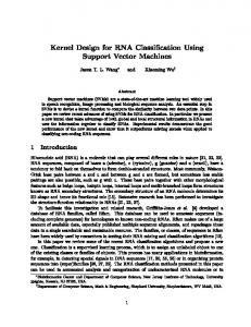
3. EXPERIMENTS We compare (i) the standard SVM with the expected kernel; (ii) the SOCP SVM using the expected kernel and the kernel variance given above; and (iii) the SOCP SVM as impleˆ ij = K(ˆ mented by its authors [5, 6] with K xi , x ˆj ) where x ˆi is an imputed estimated of xi using expectation maximization (EM) [8] and Σki = I. We consider two benchmark datasets—Ionosphere and Heart—each randomly partitioned 9:1 into disjoint training and test sets. For each dataset, we randomly set as missing 5% to 40% of the entries of each training vector. Results are averaged over 10 independent runs of the experiment. The parameters γ (for RBF kernel), C (for the SVM and SOCP SVM), and τi = τ are determined via 5-fold crossvalidation. 4. RESULTS Classification error as a function of missing feature fraction is plotted for each kernel type and dataset in Figure 1. The
=(πγ
−1 d/2
)
N (a; b, A + B + (2γ)−1 I).
(A)
Then from (3), compute the square of the expected value �2 � �2 � E K rbf (X, Y ) = γ d/2 N (a; b, A + B + γ −1 I) −1/2 =γ d/2 4π(A + B + γ −1 I) × � � � 1 −1 A+B+γ I . (B) N a; b, 2 Then, the variance of the RBF kernel in (7) is the difference of equations (A) and (B). B. REFERENCES [1] A. Farhangfar, L. Kurgan, and J. Dy, “Impact of imputation of missing values on classification error for discrete data,” Pattern Recognition, vol. 41, pp. 3692–3705, 2008. [2] J. L. Schafer and J. W. Graham, “Missing data: Our view of the state of the art,” Psychological Methods, vol. 7, no. 2, pp. 147–177, 2002.
Linear Kernels: Ionosphere
Linear Kernels: Heart
RBF Kernels: Ionosphere
RBF Kernels: Heart
Fig. 1. SVM classification error using RBF kernel for Ionosphere (left) and Heart (right). [3] H. S. Anderson, M. R. Gupta, E. Swanson, and K. Jamieson, “Channel-robust classifiers,” IEEE Trans. Sig. Proc, vol. 59, no. 4, pp. 1421. [4] H. Kashima and K. Tsuda nad A. Inokuchi, “Marginalized kernels between labeled graphs,” Proc. Intl. Conf. Machine Learning, 2003. [5] P. K. Shivaswamy, C. Bhattacharyya, and A. J. Smola, “Second order cone programming approaches for handling missing and uncertain data,” J. Mach. Learn. Res., vol. 7, pp. 1283–1314, 2006. [6] Email conversation with Pannanga Shivaswamy, January 2011. [7] G. G. Brown and H. C. Rutemiller, “Means and variances of stochastic vector products with applications to random
linear models,” Man. Sci., vol. 24, no. 2, pp. 210–216, 1977. [8] M. R. Gupta and Y. Chen, Theory and Use of the EM Method, Foundations and Trends in Signal Processing Series by NOW Publishers, 2011.