Expected Uncertain Utility Theory

Expected Uncertain Utility Theory†

Faruk Gul and Wolfgang Pesendorfer Princeton University

March 2013 Abstract We introduce and analyze expected uncertain utility theory (EUU). A prior and an interval utility characterize an EUU decision maker. The decision maker transforms each uncertain prospect into an interval-valued prospect that assigns an interval of prizes to each state. She then ranks prospects according to their expected interval utilities. We define uncertainty aversion for EUU, use the EUU model to address the Ellsberg Paradox and other ambiguity evidence, and relate EUU theory to existing models.

† This research was supported by grants from the National Science Foundation. We are grateful to Peter Wakker, Adriano Basso, Jay Lu and three anonymous referees for their comments and suggestions.

1.

Introduction We consider an agent who must choose between Savage acts that associate a mone-

tary prize to every state of nature. The agent has a prior µ on a σ−algebra E of ideal events. Ideal events capture aspects of the uncertainty that the agent can quantify without difficulty. For E−measurable acts (ideal acts) the agent is an expected utility maximizer. Therefore, the utility of an E measurable act f is ∫ W (f ) =

v(f )dµ

(1)

for some von Neumann-Morgenstern utility index v. When confronted with a non-ideal acts, f , the agent forms an ideal lower bound [f ]1 and an ideal upper bound [f ]2 . These bounds represent the range of possible outcomes implied by uncertainty that cannot be quantified. The utility of act f is ∫ W (f ) =

u ([f ]1 , [f ]2 ) dµ

(2)

where u(x, y) is the utility of an unquantifiable uncertain prospect with prizes between x and y. We refer to the utility function W as an expected uncertain utility (EUU) and to the utility index u as an interval utility. When f is ideal, the lower and upper bounds coincide and (2) reduces to the expected utility formula (1) with utility index v such that v(x) = u(x, x). The purpose of the extension to non-ideal acts is to accommodate well-documented deviations from expected utility theory. EUU theory interprets these deviations as instances in which the decision maker cannot quantify all aspects of the relevant uncertainty. EUU theory is closely tied to Savage’s model and, as a result, mirrors that model’s separation between uncertainty perception and uncertainty attitude: the prior µ measures uncertainty perception while the interval utility u measures uncertainty attitude. Despite its closeness to subjective expected utility theory, EUU is flexible enough to accommodate Ellsberg-style and Allais-style evidence. The former identifies behavior inconsistent with any single subjective prior over the event space while the latter deals with systematic violations of the independence axiom assuming preferences are consistent with a subjective probability assessment. 1

In this paper, we provide a Savage-style representation theorem for EUU theory and use it to address Ellsberg-style experiments. Section 2 introduces the model, the axioms and the representation theorem. Section 3 defines comparative measures of uncertainty aversion and the uncertainty of events and relates these measures to the parameters of the model. Just as Savage’s theorem, our representation theorem requires a rich (continuum) state space. To address experimental evidence and to relate our model to the literature it is convenient to restrict to acts that are measurable with respect to a fixed finite partition of the state space. We introduce the discrete version of EUU theory in section 4 and provide a detailed discussion of the related literature in section 5. Section 6 uses discrete EUU and the comparative measures to address Ellsberg-style evidence and section 7 shows how EUU accommodates variations of Ellsberg experiments due to Machina (2009). In a companion paper (Gul and Pesendorfer (2012)) we show how EUU can be used to address Allais-style evidence and evidence showing that, ceteris paribus, decision makers prefer uncertain prospects that depend on familiar rather than unfamiliar events.

2.

Model and Axioms The interval X = [l, m], l < m, is the set of monetary prizes and Ω is the state space.

An act is a function f : Ω → X and F is the set of all acts. For any property P, let {P} denote the set of all ω ∈ Ω at which P holds. For example, {f > g} = {ω | f (ω) > g(ω)}. For {P} = Ω, we simply write P; that is, f ∈ [x, y] means {ω | f (ω) ∈ [x, y]} = Ω. We identify x ∈ X with the constant act f = x. Consider the following 6 axioms for binary relations on F: Axiom 1:

The binary relation ≽ is complete and transitive.

Axiom 2 is a natural consequence of the fact that acts yield monetary prizes.1 Axiom 2:

If f > g, then f ≻ g.

For any f, g ∈ F and A ⊂ Ω, let f Ag denote the act that agrees with f on A and with g on the Ac , the complement of A; that is f Ag is the unique act h such that A ⊂ {h = f } 1

Though natural, the assumption is not implied by the Savage axioms and cannot be satisfied in the Savage model with a countable state space, see Wakker (1993).

2

and Ac ⊂ {h = g}. Ideal events are events E such that Savage’s sure thing principle holds for E and E c . Definition:

An event E is ideal if [f Eh ≽ gEh and hEf ≽ hEg] implies [f Eh′ ≽ gEh′

and h′ Ef ≽ h′ Eg] for all acts f, g, h and h′ . An event A is null if f Ah ∼ gAh for all f, g, h ∈ F. Let E be the set of all ideal events and E, E ′ , Ei etc. denote elements of E. Let E+ ⊂ E denote the set of ideal events that are not null. Our main hypothesis is that the agent uses elements of E+ to quantify the uncertainty of all events. More precisely, if A contains exactly the same elements of E+ as B and Ac contains the exactly the same elements of E+ as B c , then the agent is indifferent between identical bets on A and B. Axiom 3, below, formalizes this hypothesis; the axiom is weaker since it applies the hypothesis only to a subset of events but our representation implies that it holds for all events. An event is diffuse if it and its complement contains no element of E+ . Definition:

An event D is diffuse if E ∩ D ̸= ∅ = ̸ E ∩ Dc for every E ∈ E+ .

Let D be the set of all diffuse events; let D, D′ , Di etc. denote elements of D and note that they represent events whose likelihood cannot be bounded by elements of E+ . Axiom 3 requires that the decision maker is indifferent between betting on E ∩ D1 and E ∩ D2 if E ∈ E and D1 , D2 ∈ D. Notice that E ∩ D1 and E ∩ D2 contain no element of E+ while (E ∩ D1 )c and (E ∩ D2 )c both contain exactly those elements of E+ that are contained in E c . Thus, Axiom 3, below, is an implication of our main hypothesis. Axiom 3:

yE ∩ Dx ∼ yE ∩ D′ x for all x, y, E, D and D′ .

One consequence of Axiom 3 is that it permits the partitioning of Ω into a finite collections of sets D1 , . . . , Dn such that y(Dj ∪ Dk )x ∼ yDi x for all i, j and k. Note that Savage’s theory allows for a similar possibility for infinite collections of sets. Diffuse sets are limiting events that play a similar role in EUU theory as arbitrarily unlikely events do in Savage’s theory. They allow us to calibrate the uncertainty of events. Axiom 4 below is Savage’s comparative probability axiom (P4) applied to ideal events. Axiom 4:

If y > x and w > z, then yEx ≽ yE ′ x implies wEz ≽ wE ′ z. 3

Axiom 5 is Savage’s divisibility axiom for ideal events. It serves the same role here as in Savage. Its statement below is a little simpler than Savage’s original statement because our setting has a best and a worst prize. Let F o denote the set of simple acts; that is, acts such that f (Ω) is finite. The simple act, f ∈ F o , is ideal if f −1 (x) ∈ E for all x. Let F e denote the set of ideal simple acts. Axiom 5:

If f, g ∈ F e and f ≻ g, then there exists a partition E1 , . . . , En of Ω such

that lEi f ≻ mEi g for all i. Axiom 6 below is a strengthening of Savage’s dominance condition adapted to our setting. We use it to extend the representation from simple acts to all acts, to establish continuity of u and to guarantee countable additivity of the prior µ. For ideal acts f ∈ F e , Axiom 6(i) implies Arrow’s (1970) monotone continuity axiom, the standard axiom for ensuring the countable additivity of the probability measure in subjective expected utility theory. Axiom 6:

Let g ≽ fn ≽ h for all n. Then, (i) fn ∈ F e converges pointwise to f implies

g ≽ f ≽ h. (ii) fn ∈ F converges uniformly to f implies g ≽ f ≽ h. Axiom 6(ii) is what would be required to get a continuous von Neumann-Morgenstern utility index when proving Savage’s Theorem in a setting with real-valued prizes. Here, it serves a similar role; it ensures the continuity of the interval utility. Theorem 1 below is our main result. It establishes the equivalence of the six axioms to the existence of an EUU representation. The EUU representation has two parameters, a prior µ and an interval utility u that assigns a utility to a prize interval. A countably additive probability measure µ on some σ−algebra Eµ is a prior if it is complete and nonatomic.2 Let I = {[x, y] | l ≤ x ≤ y ≤ m} be the set of all prize intervals. Given any function u : I → IR, we write u(x, y) rather than the more cumbersome u([x, y]). Such a function is an interval utility if it is continuous and u(x, y) > u(x′ , y ′ ) whenever x > x′ and y > y ′ . A prior is complete if A ⊂ E and µ(E) = 0 implies A ∈ Eµ . It is non-atomic if µ(A) > 0 implies 0 < µ(B) < µ(A) for some B ⊂ A. 2

4

Let Fµ be the set of all Eµ -measurable acts and let Fµ be the set of Eµ -measurable functions f : Ω → I. We refer to elements of Fµ as interval acts. For f ∈ F, let fi denote the i’t coordinate of f so that f(ω) = [f1 (ω), f2 (ω)], f1 (ω) ≤ f2 (ω) and fi ∈ Fµ . Definition:

The interval act f ∈ Fµ is the envelope of f ∈ F if (i) f ∈ f and (ii) f ∈ g

and g ∈ Fµ imply µ{f ⊂ g} = 1. By definition, f ’s envelope, if it exists, is unique up to sets of measure zero.3 Lemma 1 below shows that every act has an envelope and that the mapping from acts to envelopes is onto.4 Lemma 1:

Fix a prior µ. Then, every act f ∈ F has an envelope and, conversely, for

any f ∈ Fµ , there is f ∈ F such that f is f ’s envelope. Henceforth, we let [f ] = ([f ]1 , [f ]2 ) denote the envelope of f . A preference ≽ is an expected uncertain utility (EUU) if there exists a prior µ and an interval utility u such that the function W defined as

∫ W (f ) =

u[f ]dµ

(3)

represents ≽. We write W = (µ, u) if W, u, µ satisfy equation (3) and let ≽uµ denote the EUU preference associated with (µ, u). Theorem 1:

The binary relation ≽ satisfies Axioms 1 − 6 if and only if there is a prior

µ and an interval utility u such that ≽ = ≽uµ . Routine arguments ensure that the prior is unique and the interval utility is unique up to a positive affine transformation for any ≽uµ . The set of ideal events E for ≽uµ is the σ−algebra Eµ .5 Hence, Fµ is the set of ideal acts F e and, since [f ]1 = [f ]2 = f for f ∈ Fµ , the restriction of ≽ to ideal events is a subjective expected utility preference . In subjective expected utility theory, the prior measures the decision maker’s uncertainty perception. With it any act can be mapped to a lottery over prizes such that the 3

In probability theory, the standard term for [f ]1 is maximal measurable minorant of f and [f ]2 is the minimal measurable majorant (van der Waart and Wellner (1996)). We use the more concise term envelope for the pair [f ]1 , [f ]2 for brevity. 4 To establish that for every envelope there is an act with that envelope, we use the Banach-Kuratowski theorem (Birkhoff (1967)) which uses the continuum hypothesis. The continuum hypothesis is needed for the Lemma to hold for any prior. However, in particular examples of priors, such as the example below, the Lemma can be verified directly. 5 See Lemma B11 for a proof of this assertion.

5

utility of the act is equal to the expected utility of the lottery. EUU allows an analogous two-step evaluation of acts. With the prior each act can be mapped into a lottery over prize intervals such that the utility of the act is equal to the expected utility of the interval lottery. For any set Y , a probability on Y is a function q : Y → [0, 1] such that {y : q(y) > 0} ∑ is a finite set and Y q(y) = 1. An interval lottery is a probability on I. Let Λ be the the set of interval lotteries. For the prior µ and the simple act f ∈ F o , let λfµ := µ ◦ [f ]−1 ; that is, λfµ (x, y) = µ{f = [x, y]} for all [x, y] ∈ I. Then, ∫ u[f ]dµ =

∑

u(x, y)λfµ (x, y)

I

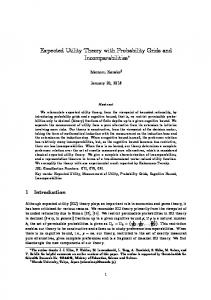
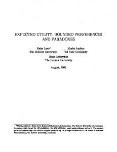
The following example illustrates the mapping from acts to envelopes and interval lotteries. Example: Let Ω = [0, 1] × [0, 1] be the unit square and let E0 be the smallest σ-algebra that contains all events of the form [a, b] × [0, 1] for 0 ≤ a ≤ b ≤ 1. That is, E0 contains all full-height rectangles as illustrated by the set E in the left hand panel of Figure 1 below. The set A depicted in the same figure is not an element of E0 .

E

A

A E1

E2

E3

Figure 1 Let µ0 be the unique measure on E0 that satisfies µ0 [a, b] × [0, 1] = b − a and let the agent’s prior, µ, be the completion of (E0 , µ0 ).6 For example, the act fˆ = xEy is ideal and has utility W (fˆ) = µ(E)u(x, x) + (1 − µ(E))u(y, y). 6

Therefore, if B is a (Lebesgue-)measure zero subset of [0, 1], then any subset of B × [0, 1] is in Eµ .

6

Next, consider the (not ideal) act f = xAy, where x < y and A is the set depicted in the right panel of Figure 1. The act f yields prize x on the light shaded region and y on the dark shaded region. The envelope of f is [f ]1 = xE1 ∪ E2 y, [f ]2 = xE1 y where the sets E1 , E2 and E3 as depicted in the right panel of Figure 1. Therefore, the utility of f is W (f ) = u(x, x)µ(E1 ) + u(x, y)µ(E2 ) + u(y, y)µ(E3 ). The interval lottery λfµ assign probability µ(E1 ) to (x, x), µ(E2 ) to (x, y) and µ(E3 ) to (y, y) and, thus, the utility of f can be written as the expected utility of the interval lottery λfµ : W (f ) = u(x, x)λfµ (x, x) + u(x, y)λfµ (x, y) + u(y, y)λfµ (y, y) .

3.

Attitude and Perception In expected utility theory, the prior describes an agent’s risk perception; that is, it

determines how each act gets mapped to a lottery. The prior plays the same role in EUU; it determines how each act is mapped to an interval lottery. The mapping from acts to interval lotteries is onto just like the mapping from acts to lotteries in Savage’s model. That is, given any prior, any interval lottery can be generated by some simple act. Lemma 2:

For any λ ∈ Λ and prior µ, there is f ∈ F o such that λfµ = λ.

Lemma 2 implies that, irrespective of the prior, each EUU decision maker confronts the same range of prospects. For any pair of priors µ and µ ¯ and any act f ∈ F o we can ¯ ¯ perceives the same risk and find f¯ ∈ F o such that λfµ = λfµ¯ . Thus, the agent with prior µ

uncertainty from act f¯ as the agent with prior µ does from act f . This enables EUU to compare the attitudes of agents with different priors. The EUU preferences ≽uµ and ≽uµ¯¯ ¯

have the same attitude if λfµ¯ = λfµ , λgµ¯¯ = λgµ implies f ≽uµ g if and only if f¯ ≽uµ¯¯ g¯ Lemma 3 below shows how the EUU model achieves separation between uncertainty perception and attitude: Consider two EUU agents with identical priors. How these agents rank acts depends only on their uncertainty attitudes (i.e., interval utilities). When the 7

two agents have different priors µ, µ ¯, we can still isolate the uncertainty attitude by controlling for the uncertainty they perceive (λµ = λµ¯ ). Lemma 3 establishes that two agents have the same uncertainty attitude if and only if one’s interval utility is a positive affine transformation the each other’s. Lemma 3:

The preference ≽uµ has the same attitude as ≽uµ¯¯ if and only if u ¯ = β1 u + β2

for some β1 , β2 ∈ IR with β1 > 0. It follows from Lemmas 2 and 3 that each interval utility u induces a preference relations ≽u on Λ. That is, λ ≽u λ′ if and only if for all µ, f, g, λfµ = λ and λfµ = λ′ implies f ≽uµ g. Henceforth, we will call this preferences the attitude ≽u . Definition:

The attitude ≽u is more cautious than ≽u¯ if x ≽u¯ λ implies x ≽u λ.

For the interval utility u, let vu (x) = u(x, x). Hence, vu : X → IR is a vNM utility index on I. For x, y ∈ X such that x < y, let σuxy be the unique σ ∈ [0, 1] that satisfies u(x, y) = vu (σx + (1 − σ)y) The quantity σuxy x + (1 − σuxy )y is the certainty equivalent of the uncertain interval [x, y]; σuxy is well defined because vu is strictly increasing, continuous and satisfies 0 ≤ σuxy ≤ 1. Theorem 2:

The attitude ≽u is more cautious than ≽u¯ if and only if vu ◦ vu−1 ¯ is concave

and σuxy ≥ σuxy ¯ for all x < y. Suppose ≽u and ≽u¯ are equally cautious; that is, each is (weakly) more cautious than the other. Then, Theorem 2 ensures that both vu ◦ vu−1 and its inverse are concave and ¯ xy u u ¯ xy therefore vu ◦ vu−1 ¯ for all x < y and therefore ≽ =≽ . Hence, ¯ is affine. Also, σu = σu

similar to expected utility theory, two individuals that have the same level of cautiousness (risk aversion in expected utility theory) have the same ranking of interval lotteries (regular lotteries in expected utility theory). The function vu describes the interval utility for degenerate intervals [x, x]. As Theorem 2 shows, the more cautious preference has a more concave vu . This part of the comparative measure corresponds to the standard comparative measure of risk aversion for expected utility maximizers. For non-degenerate intervals, the more cautious interval 8

utility has a lower certainty equivalent than the less cautious interval utility. This is the novel part that generalizes risk aversion to include uncertainty aversion. Next, we separate uncertainty aversion from risk aversion. To do so, take advantage of an insight from Epstein (1999) and use ideal acts (and diffuse acts) as benchmarks.7 Recall that F e are the ideal acts. Let Λe = {λ ∈ Λ | λfµ for f ∈ F e }. Hence, Λe is the set of ideal interval lotteries; that is, the set of all interval lotteries that can be generated by ideal acts. By using ideal interval lotteries as benchmarks, we can identify the decision-makers uncertainty attitude. Definition:

The attitude ≽u is more uncertainty averse than ≽u¯ if λ ≽u¯ λ′ implies

λ ≽u λ′ for all λ ∈ Λe . Our definition differs from Epstein’s (1999) since it accommodates differences in priors by comparing acts that yield the same interval lottery. The following Corollary to Theorem 2 characterizes comparative uncertainty aversion. In particular, it establishes that one attitude is more uncertainty averse than another if and only if it is more cautious than the other and the two have the same ranking of ideal acts. Corollary 1:

The attitude ≽u is more uncertainty averse than ≽u¯ if and only if ≽u is

more cautious than ≽u¯ and vu is a positive affine transformation of vu¯ . Next, we use our comparative measure of uncertainty aversion to derive a comparative measure for the uncertainty of events. First, fix a prior µ and consider two events A, B ⊂ Ω. If, for every interval utility u, the EUU preference ≽uµ prefers betting on B to betting on A, then B is a better bet; that is, B dominates A. Definition:

Event B dominates A if x < y implies yBx ≽uµ yAx for every interval utility

u; A and B are comparable if neither dominates the other. Between any two ideal events, the one with the higher probability will dominate the other and hence two different EUU decision-makers always rank bets on ideal events the 7

Epstein (1999) uses as a benchmark a subset of acts for which the agent is probabilistically sophisticated but not necessarily an expected utility maximizer. Ghirardato and Marinacci (2002) consider an Anscombe-Aumann setting and use objective lotteries as a benchmark. Our definition uses ideal acts as a benchmark. The difference between our comparative notion and the ones of Epstein (1999) and Ghirardato and Marinacci (2002) is that we adjust for differences in uncertainty perception and, therefore, our comparative measure applies even when agents have different priors.

9

same way. With non-ideal events, it is possible for some EUU decision-makers to prefer betting on A while others with the same perception of uncertainty prefer betting on B. This difference in behavior reflects the difference in the decision-makers’ uncertainty attitude and the differing levels uncertainty associated with these events. If more uncertainty averse u’s prefer B to A while less uncertainty averse ones have the opposite ranking, then we say A is more uncertain than B. Definition: Event A is more uncertain than B if A and B are comparable and if x < y, ≽u1 more uncertainty averse than ≽u2 , and yBx ≽uµ2 yAx imply yBx ≽uµ1 yAx. For any A ⊂ Ω the inner probability of the event A is defined as: µ∗ (A) = sup µ(E) E∈Eµ E⊂A

For ideal events µ∗ (E) + µ∗ (E c ) = 1 while for general events µ∗ (A) + µ∗ (Ac ) ≤ 1. Theorem 3: Event B dominates A if and only if µ∗ (A) ≤ µ∗ (B) and µ∗ (Ac ) ≥ µ∗ (B c ); A is more uncertain than B if and only if µ∗ (A) < µ∗ (B) and µ∗ (Ac ) < µ∗ (B c ). The difference 1 − (µ∗ (A) + µ∗ (Ac )) represents the probability mass the agent cannot distribute to A or to Ac . Theorem 3 shows that when A is more uncertain than B, this difference is greater for A than for B.

4.

EUU in a Discrete Setting To prove Theorem 1 above, we require an infinite state space. However, in applications

and when comparing the EUU model to existing alternatives, it is convenient to use a discrete state space. Let S = {1, . . . , n} be the finite state space, P be the set of nonempty subsets of S and let a, a′ , b, b′ etc. denote elements of P. We interpret S as a partition of the original state space Ω. The onto function ρ : Ω → S describes this partition so that state s in the discrete model corresponds to the event ρ−1 (s) ⊂ Ω in the original model. With slight abuse of terminology, we refer to ρ as a partition of S and ∪ define ρ−1 (a) := s∈a ρ−1 (s). Let ϕ : S → [l, m] be a discrete act and let Φ be the set of 10

discrete acts. The act ϕ ∈ Φ in the discrete model corresponds to the act f = ϕ ◦ ρ in the original model. As in the original model, the utility function for the discrete state space has two parameters, the interval utility u and a probability that reflects the agent’s prior in the discrete model. To see how the discrete prior is derived from the original prior, consider the case with two states S = {1, 2}: the event A = ρ−1 (1) ⊂ Ω corresponds to state 1 and Ac corresponds to state 2. The act ϕ(1) = x, ϕ(2) = y in the discrete model corresponds to xAy in the original model. As illustrated in the right panel of Figure 1 above, the expected uncertain utility depends on the probability of three events; the event E1 is the maximal ideal subset of A; the event E3 is the maximal ideal subset of Ac and the ideal set E2 represents the residual. The values µ(E1 ), µ(E2 ) and µ(E3 ) define a probability π on the non-empty subsets of S = {1, 2} where π{1} = µ(E1 ) π{2} = µ(E3 ) π{1, 2} = µ(E2 ) An agent with prior µ cannot apportion the probability µ(E2 ) to event A or event Ac . The probability π{1, 2} in the discrete model corresponds to µ(E2 ) of the original model, i.e., the part of the probability of the event {1, 2} that cannot be apportioned to state 1 or to state 2. For x < y, the utility of the discrete act ϕ is U (ϕ) = π{1}u(x, x) + π{1, 2}u(x, y) + π{2}u(y, y) For the general case with n ≥ 2, let P be the set of all nonempty subsets of S and let Π be the set of all probabilities on P. A preference ≽ (on Φ) is a discrete EUU if it there an interval utility u and a probability π ∈ Π such that U (ϕ) =

∑ a∈P

u(min ϕ(s), max ϕ(s))π(a) s∈a

s∈a

(4)

represents ≽. Henceforth, write U = (u, π) if U, π, u satisfy equation (4) and we let ≽uπ denote the discrete EUU that this U represents. 11

Theorem 4:

Fix W = (u, µ), S and for any π ∈ Π, let Uπ = (u, π). Then, for every

partition ρ, there is a unique π such that W (ϕ ◦ ρ) = Uπ (ϕ) for all ϕ ∈ Φ. Conversely, for every π, there is a partition ρ such that W (ϕ ◦ ρ) = Uπ (ϕ) for all ϕ ∈ Φ. Theorem 4 shows that the prior µ in the original model does not constrain the prior π in the discrete model. For any π ∈ Π, there is a partition that generates this prior. One special case is the discrete prior corresponding to a partition of the original state space into ideal subsets. In that case, π(a) = 0 for all non-singleton a and U (ϕ) =

∑

vu (ϕ(s))π{s}

s∈S

Thus, U = (u, π) is an expected utility function. If π(a) > 0 for some non-singleton a, the quantity π(a) reflects the decision maker’s inability to reduce the uncertainty of the event a to uncertainty about its components. Given any probability π on P, define the capacity8 π∗ such that π∗ (∅) = 0 and for all a ⊂ S π∗ (a) =

∑

π(b)

b∈P, b⊂a

The prior π corresponding to partition ρ satisfies ( ) π∗ (a) = µ∗ ρ−1 (a) for all a ∈ P. The co-capacity π ∗ of π∗ is defined as π ∗ (a) = 1 − π∗ (ac ) for all a ⊂ S. Note that π ∗ (a) =

∑

( ) π(b) = 1 − µ∗ ρ−1 (ac )

b∈P, b∩a̸=∅

The functions π, π∗ , π ∗ are the central concepts of Dempster-Shafer theory (Dempster (1967), Shafer (1976)). The probability π is called a basic belief assignment; the capacity π∗ is a belief function and interpreted as a lower bound on the probability of event a; π ∗ is the plausibility function and interpreted as an upper bound on the probability of the event 8

A function κ is a capacity if (i) κ(∅) = 0, κ(S) = 1 and (ii) a ⊂ b implies κ(a) ≤ κ(b).

12

a. Let ∆S be the set of all probabilities on S and let ∆π ⊂ ∆S be the core of the capacity π∗ .9 That is,

{ ∆π =

p ∈ ∆S | π∗ (a) ≤

∑

} p(s) for all a ⊂ S

s∈a

Theorem 3 describes how the discrete prior, π, measures the uncertainty of events. Translated to the discrete setting, Theorem 3 implies the following Corollary: Corollary 2:

Event a is more uncertain than event b if and only if π∗ (b) > π∗ (a) and

π ∗ (a) > π ∗ (b). Thus, in the language of Dempster-Shafer theory, event a is more uncertain than event b if it has a greater gap between belief and plausibility. For example, assume there are three states, S = {1, 2, 3} and π{1} = 1/3, π{2} = π{3} = α ∈ [0, 1/3) and π{2, 3} = 2/3. State 1 is ideal since π∗ {1} = 1/3 = π ∗ {1} and, since π∗ ({2}) = α, π ∗ {2} = 2/3 − α, state 2 is more uncertain than state 1. Our next result relates EUU to Choquet expected utility (Schmeidler (1989)) and to α-maxmin expected utility. A binary relation ≽ on Φ is a Choquet expected utility (CEU) preference if there exist a capacity κ and a continuous strictly increasing function ∫ v : X → IR such that the function V : Φ → IR defined by V (ϕ) = v(ϕ)dκ represents ≽, where the integral above denotes the Choquet integral. We write ≽κv for a CEU preference ∫ with parameters κ and v and V = (v, κ) if V (ϕ) = v(ϕ)dκ for all ϕ. For α ∈ [0, 1], the binary relation ≽ on Φ is an α-maxmin expected utility (α-MEU) preference if there exists a compact set of probabilities ∆ ⊂ ∆S and a continuous strictly increasing v : X → IR such that the function V defined by V (ϕ) = α min p∈∆

∑

v(ϕ(s))p(s) + (1 − α) max p∈∆

s∈S

∑

v(ϕ(s))p(s)

s∈S

represents ≽. We let ≽α∆v denote the α-MEU with parameters α, ∆, v and write V = (v, ∆, α) if the equation above holds for all ϕ. Theorem 5 gives a condition on the interval utility so that the EUU preference is in the intersection of CEU and α-MEU preferences. 9

See Schmeidler (1989) for a definition of the core of a capacity. Schmeidler shows that every convex capacity has a non-empty core. Since π∗ is convex it follows that ∆π is nonempty.

13

Theorem 5:

Let v : X → IR be is a continuous, strictly increasing function, α ∈ (0, 1)

and u(x, y) = αv(x) + (1 − α)v(y) for all (x, y) ∈ I. Then, ≽κv = ≽α∆v = ≽uπ for κ = απ∗ + (1 − α)π ∗ and ∆ = ∆π . Theorem 5 shows that when u is separable with the same utility index applied to the upper and lower bounds of the interval, EUU coincides with CEU and α−MEU. When α = 1, the interval utility depends only on the lower bound and hence the discrete EUU preference coincides with the MEU preference (Gilboa-Schmeidler (1989)) with utility index vu and the set of probabilities ∆π . Theorems 4 and 5 can be combined to establish conditions under which a CEU or an α−MEU is a discrete EUU: If ≽κv is a CEU with a capacity that can be expressed as a convex combination of a belief function and its plausibility function, then ≽κv is a discrete EUU. Similarly, if ≽α∆v is an α−MEU with a set of probabilities that form the core of a belief function, then ≽α∆v is a discrete EUU. We can apply our measure of uncertainty aversion to the preferences characterized in Theorem 5. For u(x, y) = αv(x) + (1 − α)v(y), the parameter α measures uncertainty aversion. Since v(σuxy x + (1 − σuxy )y) = αv(x) + (1 − α)v(y) it follows that σ xy increases as α increases . Therefore, (α, v) is more uncertainty averse than (¯ α, v) if α ≥ α ¯.

5.

Uncertainty and the Ellsberg Paradox In this section, we relate EUU theory to observed behavior in various versions of the

Ellsberg experiment. Our goal is not only to show that EUU theory is flexible enough to accommodate the Ellsberg paradox but also to take advantage of the separation between uncertainty perception and uncertainty attitude to relate a decision maker’s propensity for Ellsberg-paradox behavior to his uncertainty aversion parameter. The Ellsberg experiment has two possible prizes y = 1 and x = 0. Given any event b ⊂ S, a bet is an act that delivers 1 if b occurs and 0 otherwise. Hence, we can identify 14

each act with an event b. The experimenter elicits the decision makers’ preferences over some collection of bets: B ⊂ 2S . Let U = (u, π) be a discrete EUU utility. In the Ellsberg experiment, the interval utility affects behavior only through the values u(0, 0), u(1, 1) and u(0, 1). We normalize u(1, 1) = 1, u(0, 0) = 0 and u(0, 1) = z. Recall that z measures the agent’s uncertainty aversion: lower values of z correspond to greater uncertainty aversion. Since the preference depends only on π and z we write ≽zπ rather than ≽uπ . The subjects are told that one or more urns have each been filled with a fixed number of balls of various colors. An outcome is a configuration (one color for each ball in each urn) and a draw from each urn. Let S = {sit } where t = 1, . . . , k and i = 1, . . . m, the state sit ∈ S represents an outcome in which the balls were drawn from urns filled according to the t’th configuration. Let n = mk be the number of states. For example, in the single-urn experiment one ball is drawn from an urn that contains 3 balls. It is known that exactly one ball is red and the remaining 2 balls are either white or green. Let S = {sit } for i = 1, 2, 3, t = 1, 2, 3, 4. Suppose the three balls are numbered 1, 2, 3 and ball 1 is always red. Each column, t, depicts one possible color configuration and each row corresponds to a particular ball, 1, 2, or 3 being drawn. Table 1, below, describes the map from states to color draws:

config. 1

config 2

config 3

config. 4

ball 1

r

r

r

r

ball 2

w

w

g

g

ball 3

w

g

w

g

Table 1: Single Urn Experiment

In the two-urn experiment, urn I contains one red ball (ball 1) and one white ball (ball 2); urn II contains two balls that are red or white. One ball is drawn from each urn. Table 2 depicts the two-urn experiment. A column of Table 2 represents a color choice for balls 1 and 2 in urn II. For example, in column 1 both balls are white; in column 2, ball 1 is red and ball 2 is white, etc. A row represents pair of draws (balls 1 or 2) one from each urn. 15

config. 1

config 2

config 3

config. 4

ball 1 from I, ball 1 from II

rw

rr

rw

rr

ball 1 from I, ball 2 from II

rw

rw

rr

rr

ball 2 from I, ball 1 from II

ww

wr

ww

wr

ball 2 from I, ball 2 from II

ww

ww

wr

wr

Table 2: Two Urn Experiment

Let B be all combinations of color draws in S. For example, in the single urn experiment B is the algebra generated by the partition {r, w, g} while in the two-urn experiment B is the algebra generated by the partition {rr, rw, wr, ww}. We say that two events are (experimentally) comparable if they contain the same number of states. For example, the single color events r, w and g are all comparable in the single urn experiment because each contains four states. The defining feature of an Ellsberg experiment is that, for some events a ∈ B, the chance of winning at a in each configuration of the urn is fixed. For example, ex post (i.e., upon inspecting the contents of the urn) a = g ∪ w has a 2/3 chance of winning in every configuration in the single urn experiment. We call such events experimentally unambiguous. In contrast, a bet on b = r ∪ g has a 2/3 chance of winning in two configurations, a 1/3 chance in one configuration and is a sure winner in the final configuration. Hence, b is experimentally ambiguous in the single-urn experiment. Let |a| denote the cardinality of the set a and B be the algebra of subsets of S corresponding to all combinations of color draws. For any event a, let at = {s ∈ a | s = sit for some i} be the outcomes in a associated with the t’th possible configuration. An event a ∈ B is experimentally unambiguous if mint |at | = maxt |at |; otherwise, it is experimentally ambiguous. Let A be the collection of all experimentally unambiguous events in B. It is easy to see that complements of experimentally unambiguous events are experimentally unambiguous and disjoint unions of experimentally unambiguous events are experimentally unambiguous. Hence, we have: Lemma 4:

The class A of experimentally unambiguous events is a λ−system; that is,

it contains S and is closed under complements and disjoint unions. 16

Intersections of experimentally unambiguous events need not be experimentally unambiguous. Zhang’s four-color urn describes such a situation: one ball is drawn from an urn with 2 balls; balls are red, white, green or orange. There is exactly one ball in each of the following two categories: (1) red or white and (2) red or green. It follows that there is also one ball in each of the following two categories: (3) orange or green and (4) orange or white. The following table describes Zhang’s experiment:

config. 1

config 2

config 3

config. 4

ball 1

r

o

w

g

ball 2

o

r

g

w

Table 3: Zhang’s Four Color Urn

All single-color events have two states and are experimentally ambiguous. Of the six two-color events r ∪ o and w ∪ g are experimentally ambiguous. The remaining four are experimentally unambiguous. Thus, r ∪ w and r ∪ g are experimentally unambiguous but r is not. Given B, we say that the experimentally unambiguous events A are a finite source for the preference ≽ on Φ if |a| ≥ |b|, a, b ∈ A implies a ≽ b Thus, A is a finite source means that the agent is probabilistically sophisticated (in the sense of Machina and Schmeidler (1992)) on the class of experimentally unambiguous events and the probability measure η : A → [0, 1] such that η(a) =

| a| n

represents his betting preference. Our definition of a source mirrors Epstein and Zhang’s (2001) definition of unambiguous events. Like Epstein and Zhang we require that the agent be probabilistically sophisticated over an appropriate λ−system of events. 17

The collection B is an Ellsberg experiment if there exist a ∈ A and b ∈ B\A such that |a| = |b|. Given any Ellsberg experiment B and preference ≽ on Φ, (B, ≽) is an Ellsberg Paradox if A is a source for ≽ and if |a| = |b|, a ∈ A, b ̸∈ A implies a ≻ b Thus, (B, ≽) is an Ellsberg paradox means that probabilistic sophistication fails when the agent compares experimentally ambiguous and unambiguous events. Theorem 6, below, shows that for any Ellsberg experiment, there is an uncertainty perception π that renders each experimentally ambiguous event more π−uncertain than every comparable experimentally unambiguous event. Moreover, the experiment yields a paradox for any decision maker with that perception and greater uncertainty aversion than a benchmark. Theorem 6:

For any Ellsberg experiment, B, there are π and z ∗ > 0 such that

(i) A is a discrete source for ≽zπ for all z; (ii) b is more uncertain than a whenever a ∈ A, b ∈ B\A and |a| = |b|; (iii) (B, ≽zπ ) is an Ellsberg paradox for all z < z ∗ . For the discrete setting analyzed in this section, Theorem 6 shows that EUU theory can address Ellsberg-style evidence, including versions of the Ellsberg experiment that require that the unambiguous events do not form a σ−algebra. Specifically, Theorem 6 implies that there is a discrete prior for the Zhang-urn such that experimentally unambiguous events are a source with each of its elements less uncertain than comparable experimentally unambiguous events.10 Theorem 1 shows that the ideal events form a σ−algebra and, therefore, the experimentally unambiguous events in Zhang’s experiment cannot be ideal. However, as Theorem 6 shows, probabilistic sophistication is not confined to the ideal events; the prior can be chosen so that the agent is probabilistically sophisticated over the experimentally unambiguous events even if those events are not closed under intersection. Put differently, One example of such a prior is the following: there is α ≥ 0, β > 0 such that π(a) = α for all single color events; π(a) = α + β for all experimentally unambiguous two-color events; π(a) = 0 for all other events. 10

18

Theorem 6 shows that the existence of a σ−algebra of ideal events presents no obstacle to addressing Ellsberg-style evidence.

6. Machina Reversals The Ellsberg experiments analyzed in the previous section have only two prizes. In that case, a single parameter characterizes the interval utility and, as a result, each EUU is also a Choquet expected utility and an α−maxmin expected utility.11 Recently, Machina (2009) examined variations of Ellsberg experiments with more than two prizes and showed that Choquet expected utility theory (and related models) cannot accommodate behavior that appears plausible and even natural. In the context of EUU theory, Machina’s conjectured behavior is synonymous with the nonseparability of the interval utility u. To demonstrate this, we describe Machina’s experiment below and show that EUU can accommodate the conjectured behavior if and only if the interval utility is nonseparable. Assume a ball is drawn from an urn known to have 20 balls; 10 balls are marked 1 or 2 and 10 are marked 3 or 4. Let S = {1, 2, 3, 4} be the state space and, hence, each discrete act ϕ ∈ Φ corresponds to a vector (ϕ(1), ϕ(2), ϕ(3), ϕ(4)) ∈ X 4 . Machina (2009) observes that if ≽ is any Choquet expected utility such that (x1 , x2 , x3 , x4 ) ∼ (x2 , x1 , x3 , x4 ) ∼ (x2 , x1 , x4 , x3 ) ∼ (x4 , x3 , x2 , x1 )

(5)

for all x1 , x2 , x3 , x4 ∈ X, then we must have (x1 , x2 , x3 , x4 ) ∼ (x1 , x4 , x3 , x2 ) whenever x1 ≥ x3 ≥ x2 ≥ x4 . In particular, (20, 10, 10, 0) ∼ (20, 0, 10, 10). He notes that this indifference may be an undesirable restriction for a flexible model. Call it an M-reversal if a preference, ≽ on Φ, is not indifferent between (x1 , x2 , x3 , x4 ) and (x1 , x4 , x3 , x2 ) for some x1 ≥ x3 ≥ x2 ≥ x4 , xi ∈ X despite satisfying (5). Let Πm be collection of probabilities on the set of non-empty subsets of S that satisfy the following conditions: π{1, 2} = π{3, 4} > 0 and π(a) = 0 if a is any other two state event; π(a) = π(b) if a and b are both single state events or three state events. These conditions imply that any EUU with discrete prior in Πm satisfies (5) and that the events 11

Let 0 and 1 be the two prizes. Normalize u(0, 0) = 0 and u(1, 1) = 1; choose the utility index v such that v(0) = 0, v(1) = 1; set α = u(0, 1) and apply Theorem 5.

19

{1, 2} and {3, 4} are less π−uncertain than other two-state events. The interval utility u is separable if there are v1 , v2 : X → IR such that u(x, y) = v1 (x) + v2 (y) for all (x, y) ∈ I Theorem 7:

If π ∈ Πm , then ≽uπ has a no M-reversals if and only if u is separable.

Theorem 7 shows that Machina reversals occur if the interval utility is not separable. Experimental evidence reported in L’Haridon and Placido (2010) shows that 70% of subjects exhibit M-reversals and of those subjects roughly 2/3 prefer “packaging” the two extreme outcomes together. That is, (20, 0, 10, 10) ≻ (20, 10, 10, 0) This pattern of preference is implied by an interval utility that satisfies u(x4 , x1 ) + u(x3 , x2 ) > u(x1 , x2 ) + u(x3 , x4 ) for x1 ≥ x3 ≥ x2 ≥ x4 . EUU is not the only theory that can accommodate Machina reversals. Baillon, L’Haridon and Placido (2010) observe that Siniscalchi’s (2009) vector valued expected utility model permits them while α−maxmin expected utility and Klibanoff, Marinacci and Mukerji’s (2005) smooth model of uncertainty rule them out.

7.

Related Literature We can organize the literature on uncertainty and uncertainty aversion by grouping

models according to the extent to which uncertainty/ambiguity is built into the choice objects. At one extreme, there are papers such as Gilboa (1987), Casadesus-Masanell, Klibanoff and Ozdenoren (2000), Epstein and Zhang (2001), the current paper and a number of others that study preferences over Savage acts over an unstructured state space. At the other extreme, there are papers that introduce novel choice objects designed to incorporate uncertainty that cannot be reduced to risk. The latter models are silent on how “real-life” prospects are reduced to these choice objects; that is, they do not describe how Savage acts can be mapped to the investigated choice objects. For example, Olszewski (2007) and Ahn (2008) consider sets of lotteries and interpret sets with a single lottery as 20

situations in which the decision-maker can reduce all uncertainty to risk while sets with multiple lotteries depict Knightian uncertainty. In this latter category is Jaffray (1989) who studies preferences over belief functions over prizes.12 A belief function that assigns probability 0 to both singleton sets {x}, {y} but assigns probability 1 to the set {x, y} depicts a situation in which the decision maker knows that he will end-up with either x or y but views any remaining uncertainty as irreducible to risk. To see the relationship between Jaffray’s model and EUU theory, consider a discrete EUU ≽uπ . We can associate a capacity κ over the set of all nonempty subsets of X with each act ϕ in a natural way by letting ∑

κ(Y ) =

π(a)

{a| ϕ(a)⊂Y }

It is easy to verify that the discrete EUU ≽uπ is indifferent between two acts that yield the same capacity κ as defined above. Moreover, it can be shown that this induced preference will satisfy Jaffray’s assumptions. Hence, EUU theory and Jaffray’s model stand roughly in the same relationship as Savage’s theory and von Neumann-Morgenstern theory: one takes as given lotteries (probability distribution in vNM theory, capacities in the Jaffray model) as the choice objects, the other starts with acts, shows that each act can be identified with a lottery in a natural way and ensures that each preference (EU or EUU) over acts induces a preference over lotteries (EU or Jaffray). In between these two classes of models, there are those that partially build-in a distinction between uncertainty and risk. Segal (1990), Klibanoff, Marinacci and Mukerji (2005), Nau (2006) and Ergin and Gul (2009) achieve the desired effect by structuring the state space; in the first three papers, uncertainty resolves in two stages; the first stage represents ambiguity, the second stage risk. The remaining two papers assume that the state space has a product structure and identify one dimension with ambiguity and the other with risk. The extensive literature on ambiguity models in the Anscombe-Aumann framework also falls into this intermediate category. This literature includes Schmeidler (1989), who 12

As defined in the previous section, a belief function is a type of capacity.

21

introduces Choquet expected utility, Gilboa and Schmeidler (1989), who introduce maxmin expected utility, the generalizations of maxmin expected utility, such as α-maxmin expected utility preferences (see Ghirardato and Marinacci (2001b)), variational preferences of Maccheroni, Marinacci and Rustichini, (2006), the general uncertainty averse preferences of Cerreia-Vioglio, Maccheroni, Marinacci, and Montrucchio (2011), as well as Zhang’s (2002) model of Choquet expected utility with inner probabilities, Lehrer’s (2007) model of partially specified probabilities, and Siniscalchi’s (2009) vector expected utility theory. Theorem 5 above relates EUU to Choquet expected utility and to α−maxmin expected utility. EUU theory is also related to Zhang (2002) and Lehrer (2007). Zhang (2002) studies preferences in the Savage setting while Lehrer (2007) considers the Anscombe-Aumann framework with a finite state space. Ignoring the difference in the sets of prizes, in the state spaces, and in the underlying axioms, we can state the relationship between these two models and EUU theory as follows: each Lehrer representation can be identified with a Zhang representation (and vice versa) by identifying every partially specified probability with its inner probability extension to the set of all subsets of the state space. Then, it can be verified that every Lehrer/Zhang representation is equivalent to an EUU representation for some interval utility u such that u(x, y) = vu (x) for all x, y. Hence, Lehrer/Zhang preferences correspond to the subclass of EUU preferences for which the interval utility depends only on the lower end of the interval. Note that this is also the subclass of EUU preferences that are maxmin expected utility.

8.

Conclusion In this paper, we introduce Expected Uncertain Utility theory, an extension of sub-

jective expected utility theory to address well-known anomalies in choice behavior. By staying close to Savage’s model, EUU theory replicates one of the main achievements of Savage’s theory: the separation of uncertainty perception and uncertainty attitude. As in subjective expected utility theory, the agent’s uncertainty perception is described by a prior. In EUU theory, the prior serves two roles; it specifies which aspects of the uncertainty can be quantified and it measures the uncertainty of the those events than can be quantified. The theory uses a simple dichotomy that distinguishes perfectly quantifiable 22

and totally unquantifiable uncertainty. Nonetheless, mixing those two elements yields sufficient flexibility to address Ellsberg-style evidence and, as we show in a companion paper, Allais-style evidence.

9.

Appendix A: Preliminary Results The prior µ is convex ranged if, for every 0 < r < 1 and every E ∈ Eµ , there is

E ′ ⊂ E, E ′ ∈ Eµ such that µ(E ′ ) = rµ(E). A standard result (Billingsley (1995), p. 35) establishes that every countably additive nonatomic measure is convex-ranged. Hence, every prior is convex ranged. For the prior µ, let µ∗ (A) = sup µ(E) E∈Eµ E⊂A

Since µ is countably additive it is straightforward to show that the supremum is attained. Call E ∈ Eµ the core of A if E ⊂ A and µ(E) = µ∗ (A) and note that it is unique up to a set of measure 0. A set D is µ−diffuse if µ∗ (D) = µ∗ (Dc ) = 0. Let Dµ be the set of all µ−diffuse sets. Let E ∈ Eµ , N = {1, . . . , n} and {Ai }i∈N be a finite partition of E. Let N be the set of all nonempty subsets of N and for J ∈ N , let N (J) = {L ∈ N | L ⊂ J}. Let ∪ AJ = i∈J Ai , let C J be the core of AJ and let C N = E. The ideal split {E∗J }J∈N ⊂ Eµ {i}

of {Ai }i∈N is inductively defined as follows: E∗ |J| > 1,

:= C {i} for all i ∈ N ; for J such that 



  ∪ E∗J := C J \  E∗L  L∈N (J) L̸=J

Note that {E∗J } is a partition of E that satisfies ∑ µ∗ (AJ ) = µ(C J ) = L∈N (J) µ(E∗L ).

∪ L∈N (J)

E∗L ⊂ AJ for all J ∈ N and

For any act f ∈ F o with range {x1 , . . . , xn }, let {E∗J (f )} be the ideal split of {f −1 (xi )}. Lemma A1:

Let f ∈ F o with range {x1 , . . . , xn }. Then, f ∈ Fµ such that f(ω) =

(mini∈J xi , maxi∈J xi ) for ω ∈ E∗J (f ) is an envelope of f . 23

Proof: Let Ai = f −1 (xi ), AJ =

∪ i∈J

Ai and let C J be the core of AJ . To show that

f1 is a lower envelope first note that f (ω) = xi and ω ∈ E∗J (f ) implies i ∈ J. Hence, f1 ≤ f . Let g ∈ Fµ such that µ{g > f1 } > 0. Then, there exists J ∈ N such that ) ( µ {g > f1 } ∩ E∗J (f ) > 0. Let xj = mini∈J xi , let E = {g > f1 } ∩ E∗J (f ) and note that E ∈ Eµ since g ∈ Fµ . We claim that minω∈E f (ω) = xj thus proving that g ̸≤ f . Suppose, to the contrary, that minω∈E f (ω) = xi > xj . It follows that E ⊂ C I for I = J\{j}. ∪ From the construction of the ideal split it follows that C I = L∈N (I) E∗L (f ) and therefore E ̸⊂ E J (f ) yielding the desired contradiction. An analogous argument proves that [f ]2 is an upper envelope of f . By definition, the envelope of f is unique up to measure zero. In the following, the envelope of f , denoted [f ], refers to this equivalence class of interval acts. Lemma A2:

Assume the continuum hypothesis holds and µ is a prior. Then, Dµ is

non-empty and every D ∈ Dµ can be partitioned into D1 , D2 ∈ Dµ . Proof: Birkhoff (1967) page 266, Theorem 13 proves the following: under the continuum hypothesis, no nontrivial (i.e., not identically equal to 0), countably additive, measure such that every singleton has measure 0 can be defined on the algebra of all subsets of the continuum. We will use Birkoff’s result to establish that Ω must have a nonmeasurable subset. That is, there exists A ⊂ Ω such that A ∈ / Eµ . Since µ is convex valued we can construct a random variable, ψ, that has a uniform distribution on the interval [0, 1] on this probability space. (For example, see the construction in Billingsley (1995), proof of Theorem 20.4, p. 265.) Define µ ˆ(R) = µ(ψ −1 (R)) for every R ⊂ [0, 1]. If Eµ contains every subset of Ω, µ ˆ defines a measure on the set of all subsets of the unit interval. Moreover, since ψ has a uniform distribution, µ ˆ({x}) = 0 for all x ∈ [0, 1], contradicting Birkoff’s result. {1}

{2}

{1,2}

Let E∗ (A), E∗ (A), E∗ {1,2}

and let α = supA⊂Ω µ(E∗

(A) be an ideal split of {A1 , A2 } for A1 = A and A2 = Ac

(A)). By the argument above there exists A ⊂ Ω such that

A∈ / Eµ . Hence, α > 0. To establish that α is attained, consider a sequence of sets A(n) such that {1,2}

µ(E∗

(A(n))) > α − 24

1 n

for all n = 1, 2, . . .. Let E(n) =

∪

{1,2}

j≤n

[E(n) ∩ A(n)]\E(n − 1) and let A = {1,2}

and µ(E∗

{1,2}

(B(n))) ≥ µ(E∗

{1,2}

Ω\E∗

{1,2}

(A). Note that µ(E∗

{1,2}

there exists A such that µ(E∗

(A(j))) and set E(0) = ∅. Define B(n) = {1,2}

n

B(n). Note that E∗ {1,2}

(A(n))). Therefore, µ(E∗

{1,2}

α < 1, choose A such that µ(E∗

E∗ ∪

{1,2}

(B(n) ⊂ E∗

(A)

(A)) ≥ α as desired. If

(A)) = α and let B be any nonmeasurable subset of {1,2}

(A ∪ B)) > µ(E∗

(A)) = α, a contradiction. Hence,

(A)) = 1. Clearly, A ∈ Dµ .

Next, we will show any diffuse set can be partitioned into two diffuse sets. Let D ∈ Dµ and define Σ1 = {E ∩ D | E ∈ Eµ } and µ1 (E ∩ D) = µ(E) for all E ∈ Eµ . Since D ∈ Dµ it follows that when E ∩ D = E ′ ∩ D, E, E ′ differ by a set of measure 0. Hence, µ1 is well-defined. It is easy to check that µ1 is a prior on Σ1 . Then, repeating the previous argument yields a diffuse subset D1 of D. Then, for any E such that µ(E) > 0, we have µ1 (E ∩ D) > 0 and therefore E ∩ D1 ̸= ∅. A symmetric argument yields E ∩ (D\D1 ) ̸= ∅. Hence, D1 , D\D1 are in Dµ . 9.1

Proof of Lemma 1 Lemma 1.2.1 (pp 6-7) in van der Waart and Wellner (1996) establishes that every act

f has an envelope. It remains to show that for every interval act f ∈ F there is an act f ∈ F such that f = [f ]. Since µ is a prior, Lemma A2 implies Dµ is non-empty. Let f ∈ F and f = f1 Df2 for D ∈ Dµ . We claim that [f ] = f. Note that f1 (ω) ≤ f (ω) ≤ f2 (ω) for all ω. For any real-valued function g on Ω, if there exists E ∈ Eµ such that µ(E) > 0 and g(ω) > f1 (ω) for all ω ∈ E, then, since D is µ−diffuse, we have g(ω) > f1 (ω) = f (ω) for some ω ∈ D ∩ E. Therefore, g ∈ F and g1 (ω) ≤ f (ω) for all ω implies µ{g1 ≤ f1 } = 1. A symmetric argument yields g ∈ F and g2 (ω) ≥ f (ω) for all ω implies µ{g2 ≥ f2 } = 1.

25

10.

Appendix B: Outline of the Proof of Theorem 1 If we restrict attention to ideal events, Axioms 1-6 yield a standard expected utility

representation with a countably additive probability measure µ and a continuous utility index v : X → IR. Fix any diffuse event D and for (x, y) ∈ I, let u(x, y) = v(z) such that yDx ∼ z. Axioms 2 and 6 ensure that z ∈ [x, y] exists and therefore u is well defined. The proof of the Theorem shows that W represents ≽uµ . For this, it is enough to show that v(x∗ ) = W (f ) implies x∗ ∼ f . Consider any simple act f , let {x1 , . . . , xn } be the set of values that f takes, and assume without loss of generality that xi < xi+1 . Consider the partition {Ai | Ai = f −1 (xi ) for i = 1, . . . n} By Lemma A2, we can partition Ω into any finite number of diffuse events D1 , . . . , Dl . Since ∑ µ is nonatomic, given any α1 , . . . , αr > 0 such that i αi = 1, we can also constrtuct a partition of ideal events E1 , . . . , Er such that αi = µ(Ei ) for all i. Moreover, we construct these partition so that for all (i, j) ∈ {1, . . . , r} × {1, . . . , l}, there is some k ∈ {1, . . . , n} with Ei ∩ Dj ⊂ Ak . Let x, y be the minimal and maximal values of f on E1 . Let f1 be an act that agrees with f on E1c , takes on the values x and y on E1 and agrees with f when f is equal to x or y. That f1 has the same envelope as f follows from the definition of a diffuse event. To see that f1 is indifferent to f consider the simplest case: E1 = Ω and assume that f = xD1 (zD2 y) for some diffuse partition D1 , D2 , D3 . We use monotonicity and uniform continuity (Axioms 2 and 6(ii)) to show that f ≥ g implies f ≽ g. It follows that xD1 (zD2 y) ≽ xD1 ∪ D2 y and xD1 y ≽ xD1 (zD2 y). By Axiom 3, xD1 ∪ D2 y ∼ xD1 y and therefore xD1 ∪ D2 y ∼ xD1 (zD2 y) ∼ xD1 y. Then, by induction, f is indifferent to and has the same envelope as some act g that takes at most two values on each Ej and agrees with f whenever f takes its maximal or minimal value in Ej . Let yj and xj be these values respectively. Then, it follows from the definition of an ideal event and Axiom 3 that g is indifferent to the act h such that 26

h(ω) = zj for all ω ∈ Ej for zj such that zj ∼ yj Dxi . Since h is measurable with respect to ideal events, x∗ ∼ h ∼ g ∼ f for some x∗ such that v(x∗ ) =

∑

v(zj )µ(Ej ) =

∑

j

u(xj , yj )µ(Ej ) = W (g) = W (f )

j

as desired. The extension to all acts uses Axiom 6 and follows familiar arguments.

11.

Appendix B: Proof of Theorem 1 The proof is divided into a series of Lemmas. It is understood that Axioms 1-6 hold

throughout. Definition:

A set E left (right) ideal if f Eh ≽ gEh implies f Eh′ ≽ gEh′ (hEf ≽

hEg implies h′ Ef ≽ h′ Eg). Let E l and E r be the collection of left and right ideal sets respectively. Lemma B0:

(i) E r = {E | E c ∈ E l }. (ii) E l ∩ E r = E.

Proof: Assertion (i) is obvious as is the fact that E l ∩ E r ⊂ E. Suppose E ∈ E and assume f Eh ≽ gEh. Let f ∗ = f Eh and g ∗ = gEh. Then, f ∗ Eh = f Eh ≽ gEh = g ∗ Eh and hence f ∗ Eh ≽ g ∗ Eh. Also, hEf ∗ = h = hEg ∗ and hence hEf ∗ ≽ hEg ∗ and therefore f ∗ Eh′ ≽ g ∗ Eh′ and h′ Ef ∗ ≽ h′ Eg ∗ since E ∈ E. That is, f Eh′ = f ∗ Eh′ ≽ g ∗ Eh′ = gEh′ and hence E ∈ E l . A symmetric argument establishes that E ∈ E r and therefore E = E l ∩ E r . Lemma B1:

(i) f ≥ g implies f ≽ g. (ii) f ≻ g implies f ≻ z ≻ g for some z ∈ X.

(iii) fn , gn ∈ F , fn converges uniformly to f , gn converges uniformly to g, f ≻ g implies fn ≻ gn for large n. (iv) fn , gn ∈ F e , fn converges pointwise to f , gn pointwise to g, f ≻ g implies fn ≻ gn for some n. (v) If E ∈ E+ and y > x, then yEh ≻ xEh for all h ∈ F . (vi) If E ∈ E+ and f ∈ F , then there exists a unique cE (f ) ∈ X such that cE (f )Ef ∼ f . Proof: To prove (i), let fn =

1 nm

+ ( n−1 n )f and gn =

1 nl

+ ( n−1 n )g. Then, fn converges

to f uniformly and gn converges to g uniformly. By Axiom 2, fn ≻ gn . Then, by Axiom 6, f ≽ gn and applying Axiom 6 again yields f ≽ g as desired. To prove (ii), assume f ≻ g and let y = inf{z ∈ X | z ≽ f } and let x = sup{z ∈ X | g ≽ z}. By (i) above, x and y are well-defined. Axiom 6 ensures that y ∼ f and z ∼ g and therefore y ≻ x. Then, for z =

x+y 2 ,

we have f ≻ z ≻ g. 27

To prove (iii), let f ≻ g and apply (ii) three times to get z, y, x such that f ≻ z ≻ y ≻ x ≻ g. Axiom 6 ensures that fn ≻ y and y ≻ gn for all n large enough. Therefore, fn ≻ gn for all such n. An analogous argument proves (iv). To prove (v), consider E ∈ E+ , h ∈ F and x < y. Then, there exists f, g, h′ such that f Eh′ ≻ gEh′ which implies that mEh′ ≻ lEh′ by part (i) above. Lemma B0(ii) implies m ≻ lEm which implies y ≻ xEy by Axiom 4, which, again by Lemma B0(ii), implies yEh ≻ xEh as desired. Finally, let z = inf{x ∈ X | xEf ≽ f }. By part (i) mEf ≽ f and hence z is welldefined. Axiom 6 and part (v) of this lemma ensure that zEf ∼ f and also that y ̸= z implies yEf ̸∼ f . Hence, z = cE (f ). Lemma B2:

The collection E is a σ−field.

Proof: First, we will show that E is a field. That E ∈ E implies E c ∈ E is obvious as ˆ ∈E is the fact that ∅ ∈ E. Hence, to show that E is a field, we need to verify that E, E ˆ ∈ E. Let E1 = E\E, ˆ E2 = E\E, ˆ ˆ and E4 = Ω\{E ∪ E}. ˆ implies E ∪ E E3 = E ∩ E ˆ ∈ E l and E c , E ˆ c ∈ E l implies (i) E ∪ E ˆ ∈ El By Lemma B0, we need to show that E, E ˆ c ∈ E l ; that is, we need to show that E1 ∪ E2 ∪ E3 ∈ E l and E4 ∈ E l . and E c ∩ E ˆ ∈ E l and E c , E ˆ c ∈ E l . We will first show that E ∩ E ˆ ∈ E l. Assume that E, E ˆ ≽ gE ∩ Eh. ˆ ˆ = (f Eh)Eh. ˆ ˆ ∈ E, we have Suppose f E ∩ Eh Note that f E ∩ Eh Since E ˆ ′ ≽ (gEh)Eh ˆ ′ . Next, observe that (f Eh)Eh ˆ ′ = (f Eh ˆ ′ )E(hEh ˆ ′ ) and therefore, (f Eh)Eh ˆ ′) ≽ ˆ ′ )E(hEh ˆ ′ ) ≽ (g Eh ˆ ′ )E(hEh ˆ ′ ). Since E ∈ E, we have f E ∩ Eh ˆ ′ = (f Eh ˆ ′ )E(h′ Eh (f Eh ˆ ′ )E(h′ Eh ˆ ′ ) = gE ∩ Eh ˆ ′ and hence E3 = E ∩ E ˆ ∈ E l . Symmetric arguments ensure (g Eh that (i) Ei ∈ E l for i = 1, 2, 3, 4. In particular, E4 ∈ E l as desired. ˆ ≽ g Eh ˆ implies f (E1 ∪ E)h ˆ ∼ f Eh ˆ ≽ g Eh ˆ ∼ g(E1 ∪ E)h. ˆ If E1 is null, then f Eh Since ˆ ∈ E l , we conclude f Eh ˆ ′ ≽ g Eh ˆ ′ . Then, since E1 is null, we get f (E1 ∪ E)h ˆ ′ ∼ f Eh ˆ ′≽ E ˆ ′ ∼ g(E1 ∪ E)h ˆ ′ as desired. By symmetry, we can also assume E2 is not null. Hence, g Eh we have (ii) E1 , E2 are nonnull. Next, we will show that (iii) for all h, mE1 h ≻ lE1 h. Since E1 is nonnull, the assertion is true for some h∗ . But, since E1 ∈ E l , we conclude that mE1 h ≻ lE1 h for all h. Throughout the remainder of the proof of this lemma, we let (x1 , x2 , x3 , h) denote the act that yields xi on ω ∈ Ei for i = 1, 2, 3 and h(ω) on ω ∈ E4 . 28

Let ≽h denote following binary relation on X 3 : (x1 , x2 , x3 ) ≽h (y1 , y2 , y3 ) if (x1 , x2 , x3 , h) ≽ (y1 , y2 , y3 , h) Similarly, let x1 ≽z2 z3 h y1 if (x1 , z2 , z3 , h) ≽∗ (y1 , z2 , z3 , h); (x1 , x3 ) ≽z2 h (y1 , y3 ) if (x1 , z2 , x3 , h) ≽ (y1 , z2 , y3 , h). Define ≽z1 z2 z3 and ≽z1 h in an analogous fashion. We claim that ≽h =≽h′ for all h, h′ . Otherwise, let ≽h∗ ̸=≽h′ . Then, define the following binary relation on X 3 × [0, 1]: (x1 , x2 , x3 , α) ≽∗ (y1 , z2 , z3 , β) if and only if (x1 , x2 , x3 , αh∗ + (1 − α)h′ ) ≽∗ (y1 , y2 , y3 , βh∗ + (1 − β)h′ ). Define ≽∗α , ≽∗x1 etc. by replacing the h in the definition of ≽h , ≽x1 with α. Since ≽ is complete and transitive, Axiom 6(ii) ensures that (1) ≽ is complete, transitive and continuous. Note that (iii) implies (2) m ≻∗z2 z3 α l for all z2 , z3 , α. Finally, since (x1 , x2 , x3 , α) ≽ (y1 , y2 , y3 , α) and (y1 , y2 , y3 , β) ≻ (x1 , x2 , x3 , β) for some ˆ z 1 , z2 , z3 . ˆ , β, x1 , x2 , x3 , α, y1 , y2 , y3 , β, we must have (3) α ˆ ≻∗z1 z2 z3 βˆ for some α After some translation of terminology and interpreting the slightly stronger assumptions of the current setting, Theorem 1 in Gorman (1968) yields: Fact: If (1), (2) and (3), then ≽∗α =≽∗β for all α, β ∈ [0, 1]. The fact above contradicts our hypothesis that ≽h∗ ̸=≽h′ . So, we must have (iv) (x1 , x2 , x3 , h∗ ) ≽ (y1 , y2 , y3 , h∗ ) implies (x1 , x2 , x3 , h′ ) ≽ (y1 , y2 , y3 , h′ ). Then, suppose f (E1 ∪ E2 ∪ E3 )h∗ ≽ g(E1 ∪ E2 ∪ E3 )h∗ . Then, by Lemma B1(vi), there is x ∈ X such (x(E1 ∪ E3 )f )(E1 ∪ E2 ∪ E3 )h∗ ∼ f (E1 ∪ E2 ∪E3 )h∗ and y ∈ X such that (x, y, y, h∗ ) ∼ (x(E1 ∪E3 )f )(E1 ∪E2 ∪E3 )h∗ and therefore, (x, y, y, h∗ ) ∼ f (E1 ∪ E2 ∪ E3 )h∗ . Similarly, we can find x ˆ, yˆ such that (ˆ x, yˆ, yˆ, h∗ ) ∼ g(E1 ∪ E2 ∪ E3 )h∗ . Hence, (x, y, y, h∗ ) ≽ (ˆ x, yˆ, yˆ, h∗ ). Then, from (iv) above, we get ˆ ∈ E l , (x, y, y, h∗ ) ∼ (x(E1 ∪E3 )f )(E1 ∪E2 ∪E3 )h∗ (x, y, y, h′ ) ≽ (ˆ x, yˆ, yˆ, h′ ). But since E, E implies (x, y, y, h) ∼ (x(E1 ∪ E3 )f )(E1 ∪ E2 ∪ E3 )h and (x(E1 ∪ E3 )f )(E1 ∪ E2 ∪ E3 )h∗ ∼ f (E1 ∪ E2 ∪ E3 )h∗ implies (x(E1 ∪ E3 )f )(E1 ∪ E2 ∪ E3 )h′ ∼ f (E1 ∪ E2 ∪ E3 )h′ and therefore f (E1 ∪ E2 ∪ E3 )h′ ∼ (x, y, y, h′ ). A symmetric argument yields g(E1 ∪ E2 ∪ E3 )h′ ∼ (x, y, y, h′ ). Then, (x, y, y, h′ ) ≽ (ˆ x, yˆ, yˆ, h′ ) implies f (E1 ∪ E2 ∪ E3 )h′ ≽ g(E1 ∪ E2 ∪ E3 )h′ , proving that E1 ∪ E2 ∪ E3 ∈ E l . This completes the proof that E is a field. 29

To prove that the field E is a σ−field, it is enough to show that if Ei ∈ E and ∪ Ei ⊂ Ei+1 , then Ei ∈ E. Let Ei ⊂ Ei+1 for all i. Note that fˆEi gˆ converges pointwise ∪ ∪ ∪ ∪ ∪ to fˆ Ei gˆ for all fˆ, gˆ ∈ F. Hence, if g Ei h′ ≻ f Ei h′ or h′ Ei g ≻ h′ Ei f for some f, g, h, h′ ∈ F e , by Lemma B1(iv) above, we have gEn h′ ≻ f En h′ or h′ En g ≻ h′ En f for ∪ some n, proving that Ei ∈ E for all n implies i Ei ∈ E. Lemma B3:

There exists a finitely additive, convex-ranged probability measure µ on E

and a function v : Ω → IR such that (i) the function V : F e → IR defined by V (f ) =

∑

v(x)µ(f −1 (x))

x∈X

represents the restriction of ≽ to F e and (ii) If µ{f = g} = 1, then f ∼ g. Proof: Let ≽e be the restriction of ≽ to F e . By definition (of E), ≽e satisfies Savage’s P2. Similarly, Axiom 1 is Savage’s P1, Lemma B1(i) and (v) imply P3, Axiom 4 is P4, Axiom 2 implies P5, and Axiom 5 implies P6. Then, following Savage’s proof yields the desired conclusion. This is true despite the fact that Savage’s theorem assumes that the underlying σ−field is the set of all subsets of Ω; the arguments work for any σ−field. This proves (i). To prove (ii), note that, by hypothesis, there exists E ∈ E such that µ(E) = 1 and g = f Eg. But m ∼ mEl by part (i) and since E ∈ E, we have f Em ∼ f El. Then, Lemma B1(i) yields f = f Ef ∼ f Eg. Lemma B4:

.

The probability measure µ on E is a prior.

Proof: To show that µ is countably additive, we need to prove that given any sequence Ei ∩ such that Ei+1 ⊂ Ei for all i and E ∗ := i Ei = ∅, lim µ(Ei ) = 0. Suppose lim µ(Ei ) > 0. Then, convex-valuedness ensures the existence of E such that lim µ(Ei ) > µ(E) > 0. Hence, µ(Ei ) > µ(E) for all i; that is mEi l ≻ mEl for all i. But mEi l ∈ F e and converges pointwise to mE ∗ l. Hence, mE ∗ l ≽ mEl ≻ l. Therefore, µ(E ∗ ) > 0, a contradiction. To prove that µ is complete, we will assume µ(E) = 0 and A ⊂ E, then show that this implies f Ah ∼ h for all f ∈ F. This means that A ∈ E. By Lemma B1(i), f Ah ≽ lEh. Since, µ(E) = 0, Lemma B3 implies lEm ∼ m and since E ∈ E, we conclude that lEh ∼ mEh. But, mEh ≽ h by Lemma B1(i), so we have f Ah ≽ h. A symmetric argument, yields h ≽ f Ah and hence, f Ah ∼ h as desired. 30

Since µ is convex-ranged it is obviously nonatomic. Hence, µ is a prior. Lemma B5:

The function v is strictly increasing and continuous.

Proof: That v is strictly increasing follows from y ≻ x whenever y > x. To prove continuity, assume, without loss of generality, that v(m) = 1 and v(l) = 0 and suppose r = lim v(xn ) < v(x) for some sequence xn converging to x. Choose Er ∈ E such that µ(Er ) = r. By Lemma B3(i), x ≻ mEr l ≽ xn for n large. Therefore, x ≻ mEr l ≽ lim xn = x, a contradiction. Hence, r ≥ v(x). A symmetric argument yields v(x) ≥ r proving the continuity of v. Lemma B6:

(i) D = Dµ . (ii) For all (x, y) ∈ X 2 , there is a unique z ∈ X such that

yDx ∼ z for all D ∈ D. Proof: (i) By construction, Eµ = E and E+ = {E ∈ Eµ | µ(E) > 0}. Therefore, µ∗ (D) = µ∗ (Dc ) = 0 implies E ̸⊂ D and E ̸⊂ Dc for all E ∈ E+ and hence D ∈ D. Therefore, Dµ ⊂ D. For the reverse inclusion, note that D ∈ D implies that E ∩D ̸= ∅ and E ∩Dc ̸= ∅ for all E ∈ E+ . Since E+ = {E ∈ Eµ | µ(E) > 0}, it follows that µ∗ (D) = µ∗ (Dc ) = 0. (ii) By Axiom 3, xDy ∼ xD′ y for all D, D′ ∈ D. Hence, fix any D ∈ D and let z = sup{w ∈ X | yDx ≽ w}. Since, yDx ≽ l, by Lemma B1(i), z is well-defined. Then, Lemma B1(iii) rules out both z ≻ yDx and yDx ≻ z. Lemma B6(i) and Lemma A2 imply D ̸= ∅. Then, Lemma B6(ii) ensures that the function u : I → IR below, is well defined. Definition: Lemma B7:

For all x ≤ y, let u(x, y) = v(z) for z ∈ X such that yDx ∼ z for D ∈ D. Let D1 , . . . , Dn ∈ D be a partition of Ω, Di ⊂ {f = xi } for all i and

yi+1 ≥ yi for i ≤ n − 1. Then, f ∼ yn Dy1 for all D ∈ D. Proof: By Lemma B1(i), yn [D2 ∪ . . . ∪ Dn ]y1 ≽ f ≽ yn Dn y1 . By Axiom 3, yn [D2 ∪ . . . ∪ Dn ]y1 ∼ yn Dn y1 ∼ yn Dy1 . Lemma B8:

The function u is increasing and continuous.

Proof: Suppose yDx ∼ z and yˆDˆ x ∼ zˆ. If yˆ > y and x ˆ > x, then Axiom 2 implies zˆ ≻ z and applying Axiom 2 again yields zˆ > z as desired. If yˆ ≥ y and x ˆ ≥ x, then by Lemma B1(i), zˆ ≽ z. Then, applying Axiom 2 again yields zˆ ≥ z. 31

To prove continuity, assume yi Dxi ∼ zi for i = 1, . . . and lim(xi , yi ) = (x, y). Since X is compact, we can assume without loss of generality, that zi converges to some z. Then Lemma B1(iii) rules out yDx ≻ z and z ≻ yDx and establishes continuity. Define

∫ W (f ) =

Lemma B9:

u[f ]dµ

The function W represents the restriction of ≽ to F o .

Proof: Let {x1 , . . . , xn } be the range of f , let Ai = f −1 (xi ) and let {E∗J (f )} be an ideal split of {Ai }. Lemma A2 implies that {E∗J (f )} exists and is unique up to measure zero. Let N + (f ) = {J | µ(E∗J (f )) > 0 and |J| > 1} and Hn = {f ∈ F o | n = |N + (f )|}. The proof is by induction on Hn . Note that for f ∈ H0 W (f ) =

∑

v(z)µ(f −1 (z)) = v(x)

z∈X

for x such that µ{x = f } = 1. Hence, by Lemma B3(ii), W represents the restriction ≽ to H0 . Suppose W represents the restriction of ≽ to Hn and choose f ∈ Hn+1 . Define hf as follows: if f ∈ Hn , then hf = f ; otherwise, choose E∗J (f ) such that |J| > 1 and µ(E∗J (f )) > 0, choose D ∈ D and define f ∗ as follows:  if ω ∈ / E∗J (f )  f (ω) ∗ J f (ω) = max f (E∗ (f )) if ω ∈ D ∩ E∗J (f )  min f (E∗J (f )) if ω ∈ Dc ∩ E∗J (f ) By Lemma B7 and Axiom 3, f ∗ ∼ f . Next, choose z such that u(x, y) = v(z) and let hf (ω) = f ∗ (ω) for all ω ∈ / E∗J (f ) and hf (ω) = z for all ω ∈ E∗J (f ). Again, Axiom 3 ensures that hf ∼ f ∗ ∼ f . Note that hf ∈ Hn and, by construction, W (hf ) = W (f ∗ ). By Lemma A1, [f ∗ ] = [f ] and therefore W (f ∗ ) = W (f ). Thus, W (f ) = W (hf ) for some hf ∈ Hn such that hf ∼ f . Then, the induction hypothesis implies that W represents ≽ on Hn+1 .

Lemma B10:

The function W represents ≽.

Proof: Note that for all f , there exists xf such that W (xf ) = u(xf , xf ) = W (f ). This follows from that fact that u is continuous and u(m, m) ≥ W (f ) ≥ u(l, l). Hence, by the 32

intermediate value theorem u(xf , xf ) = W (f ) for some xf ∈ [l, m]. The monotonicity of u ensures that this xf is unique. Next, we show that f ∼ xf . Without loss of generality, assume l = 0 (if not let l∗ = 0 and m∗ = m − l and identify each f with f ∗ = f − l and apply all previous results to acts F ∗ = {f − l | f ∈ F }.) Define for any x ≥ 0 and ϵ > 0, z ∗ (x, ϵ) = min{nϵ | n = 0, 1, . . . such that nϵ ≥ x}. Similarly, let z∗ (x, ϵ) = max{nϵ | n = 0, 1, . . . such that nϵ ≤ x}. Clearly, 0 ≤ z ∗ (x, ϵ) − x ≤ z ∗ (x, ϵ) − z∗ (x, ϵ) ≤ ϵ

(B3)

and the first two inequalities above are equalities if and only if x is a multiple of ϵ. Set f n (ω) = z ∗ (f (ω), m2−n ) and fn (ω) = z∗ (f (ω), m2−n ) for all n = 0, 1, . . .. Equation (B3) above ensures that f n ≥ f ≥ fn and f n , fn converge uniformly to f . Note also that f n , fn ∈ F o with f n ↓ f . This implies that [f n ] ↓ [f ] µ−almost surely (see van der ∫ ∫ Waart and Wellner (1996), p. 13) and therefore u[f n ]dµ → u[f ]dµ. Since f n ≥ f , we have W (f n ) ≥ W (f ) = W (xf ) for all n. Since W represents the restriction of ≽ to F o , we conclude that f n ≽ xf for all n. Then, Axiom 6 implies f ≽ xf . A symmetric argument with fn replacing f n yields xf ≽ f and therefore xf ∼ f as desired. To conclude the proof of the Lemma, suppose f ≽ g, then W (xf ) = W (f ) and W (xg ) = W (g) and xf ∼ f ≽ g ∼ xg . Since W represents the restriction of ≽ to F o , we conclude that W (xf ) ≥ W (xg ) and hence W (f ) ≥ W (g). Similarly, if W (f ) ≥ W (g) we conclude f ∼ xf ≽ xg ∼ g and therefore f ≽ g. Lemma B10 establishes sufficiency. To prove that the preference, ≽uµ , satisfies Axioms 1-6 for every prior µ and interval utility u, we first establish that Eµ = E and Dµ = D. Lemma B11:

Let E, D be the ideal and diffuse events for the preference ≽uµ . Then,

D = Dµ , E = Eµ . Proof: From the representation it is immediate that Eµ ⊂ E which, in turn, implies D ⊂ Dµ . Thus, to prove the lemma it suffices to show that E ⊂ Eµ . For A ⊂ Ω, let {1}

{2}

{1,2}

{1,2}

{E∗ , E∗ , E∗

} be the ideal split of A, Ac . If A ̸∈ Eµ , then µ(E∗

and define

) ( ) ) ( ( {1,2} {2} {1} ∪ A ∩ E∗ D1 = D ∩ E∗ ∪ D ∩ E∗ ( ) ( ) ( ) {1} {2} {1,2} D2 = Dc ∩ E∗ ∪ D c ∩ E∗ ∪ A c ∩ E∗ 33

) > 0. Let D ∈ Dµ

Note that D1 , D2 ∈ Dµ . By Lemma A2, there are Di1 , Di2 ∈ Dµ such that Di1 ∩ Di2 = ∅ {1,2}

and Di1 ∪ Di2 = Di for i = 1, 2. Let Bij = Dij ∩ E∗

for i = 1, 2, j = 1, 2 and note that

{1}

∪ B11 ∪ B12

{2}

∪ B21 ∪ B22

A = E∗ Ac = E∗ For x1 < x2 < x3 ∈ X, let g = x1 and let { f=

x3 x2 x1

if ω ∈ B11 if ω ∈ B12 ; h = otherwise

{

x3 x1 x1

if ω ∈ B21 if ω ∈ B22 ; h′ = otherwise

{

x2 x2 x1

if ω ∈ B21 if ω ∈ B22 otherwise

Then, by Lemma A1, {1,2}

W (f Ah′ ) = µ(E∗

{1,2}

W (f Ah) = µ(E∗

{1,2}

W (gAh) = µ(E∗

{1,2}

W (gAh′ ) = µ(E∗

{1}

∪ E∗ )u(x1 , x1 )

{1}

∪ E∗ )u(x1 , x1 )

{1}

∪ E∗ )u(x1 , x1 )

{1}

∪ E∗ )u(x1 , x1 )

)u(x2 , x3 ) + µ(E∗ )u(x1 , x3 ) + µ(E∗ )u(x1 , x3 ) + µ(E∗

)u(x1 , x2 ) + µ(E∗

{2} {2} {2}

{2}

Thus, W (gAh) ≥ W (f Ah). Also, hAf = x1 = hAg and hence W (hAg) ≥ W (hAf ). But, since u is increasing, W (f Ah′ ) > W (gAh′ ), and therefore, A is not ideal. To complete the proof, note that µ is convex-ranged since it is non-atomic. Then, verifying Axioms 1, 2 and 5 involves nothing more than repeating familiar arguments from Savage’s theorem. Given Lemma B11, Axioms 3 and 4 follow immediately from the representation. Note that for any f n ∈ F e , if [f n ] converges pointwise to [g], then W (f n ) converges to W (g). Hence, Axiom 6(i) follows from the fact that f n converges to f pointwise implies [f n ] converges pointwise to [f ] while Axiom 6(ii) follows from the fact that for any f n , if f n converges to f uniformly, then [f n ] converges pointwise to [f ].

34

12.

Appendix C: Proofs for Section 3

Proof of Lemma 2: Let λ be an interval lottery and let {(x1 , y2 ), . . . , (xn , yn )} be its support. Choose a partition E1 , . . . , En of Ω such that µ(Ei ) = λ(xi , yi ). This can be done since µ is non-atomic and, therefore, convex valued. Let f ∈ F be defined as f(ω) = (xi , yi ) for ω ∈ Ei . By Lemma 1 there exists f ∈ F such that [f ] = f. That λfµ = λ is immediate.

Proof of Lemma 3: Sufficiency is immediate. For necessity, first note that vu¯ = αvu + β for some α > 0. This follows since two expected utility maximizers have the same preferences over simple lotteries only if their utility indices are the same, up to a positive affine transformation. For every (x, y) ∈ I, there exist unique z, z¯ such that vu (z) = u(x, y) ¯ be diffuse sets for µ, µ and vu¯ (¯ z) = u ¯(x, y). Let D, D ¯ respectively; let f = xDy and ¯ and note that λf = λfµ¯¯. Since f ∼u z and f ∼u¯ z¯ it follows that z = z¯. Since f¯ = xDy µ µ µ ¯ vu¯ = αvu + β it follows that u ¯ = αu + β. Proof of Theorem 2: If vu¯ ◦ vu−1 is not concave, then familiar arguments ensure the existence of x < z < y and p ∈ (0, 1) such that pvu¯ (y) + (1 − p)vu¯ (x) > vu¯ (z) and pvu (y)+(1−p)vu (x) < vu (z). Let λ be the interval lottery that yields (y, y) with probability p and (x, x) with probability 1 − p. Lemma 2 implies that there are f, f¯ such that λfµ = ¯ λfµ¯ = λ. Since f¯ ≻uµ¯¯ z and z ≻uµ f , ≽uµ¯¯ is not more uncertainty cautious than ≽uµ . xy If σuxy ¯ < σu , then choose σ strictly between these two numbers. Let λ be the interval

lottery that yields (x, y) with probability 1. Lemma 2 implies that there are f, f¯ such that ¯ λfµ = λfµ¯ = λ. Since f¯ ≻uµ¯¯ σx + (1 − σ)y and σx + (1 − σ)y ≻uµ f it follows that ≽uµ¯¯ is not

more uncertainty cautious than ≽uµ . ≥ σuxy for all x, y and vu¯ ◦ vu−1 is concave. Let To prove sufficiency, assume σuxy ¯ f ∈ F o and let λ = λfµ with support {(x1 , x2 ), . . . , (xn , yn )}. For each (xi , yi ), define zi = σux¯ i yi xi +(1−σux¯ i yi )yi . Let λ∗ be the interval lottery with support {(z1 , z1 ), . . . (zn , zn )} such that λ∗ (zi , zi ) = λ(xi , yi ) ∗

¯

¯∗

By Lemma 2, there are f ∗ , f¯, f¯∗ ∈ F o such that λfµ = λ∗ , λfµ¯ = λ and λfµ¯ = λ∗ . Note xy −1 that f¯ ∼uµ¯¯ f¯∗ by construction and f ≽uµ f ∗ since σuxy ¯ ◦ vu is concave, ¯ ≥ σu . Since vu

35

vu (z) ≥

∑n i=1

vu (zi )λ∗ (zi , zi ) implies vu¯ (z) ≥

∑n i=1

vu¯ (zi )λ∗ (zi , zi ). We conclude that

z ≽uµ f ∗ implies z ≽uµ¯¯ f¯∗ ∼uµ¯¯ f¯. Since f ≽uµ f ∗ , it follows that z ≽uµ f implies z ≽uµ¯¯ f¯ as desired. Proof of Corollary 1: The proof is straightforward and therefore omitted. Proof of Theorem 3: Let f = xAy be a binary act with x < y. We first show that if W = (u, µ), then W (yAx) = µ∗ (A)u(y, y) + µ∗ (Ac )u(x, x) + (1 − µ∗ (A) − µ∗ (Ac ))u(x, y)

(∗)

{ } {1} {2} {12} Let A1 = A, A2 = A and E∗ , E∗ , E∗ be the ideal split of A1 , A2 . Then, by c

Lemma A1 and the definition of an ideal split it follows that ( ) {1} {12} [f ]1 = x E∗ ∪ E∗ y ( ) {1} [f ]2 = x E∗ y ( ) {i} where µ E∗ = µ∗ (Ai ) for i = 1, 2. Applying the representation now proves the assertion. Then, let u(x, y) = x and u∗ (x, y) = y. If µ∗ (A) > µ∗ (B), the assertion above yields ∗

yAx ≻u yBx; if µ∗ (Ac ) < µ∗ (B c ); the assertion above yields yAx ≻u yBx. Hence, B dominates A implies µ∗ (A) ≤ µ∗ (B) and µ∗ (Ac ) ≤ µ∗ (B c ). Conversely, if µ∗ (A) ≤ µ∗ (B), µ∗ (Ac ) ≤ µ∗ (B c ), the assertion above ensures that yBx ≻uˆ yAx for all u ˆ. Suppose A is more uncertain than B and let u, u∗ , W, W ∗ be as above. Suppose A, B are comparable so that [µ∗ (B) − µ∗ (A)] · [µ∗ (Ac ) − µ∗ (B c )] < 0. Then choose z such that x < z < y and [µ∗ (B) − µ∗ (A)][y − z] + [µ∗ (Ac ) − µ∗ (B c )][z − x] = 0 Let t =

y−z y−x

and u ˆ(x′ , y ′ ) = tx + (1 − t)y for all (x′ , y ′ ) ∈ I. Note that ≽u is more ′

uncertainty averse than ≽u and therefore, we must have [µ∗ (B) − µ∗ (A)][y − x] ≥ 0 36

That is, we must have µ∗ (B) − µ∗ (A) > 0 and µ∗ (Ac ) − µ∗ (B c ) < 0. Conversely, assume µ∗ (B) − µ∗ (A) > 0, µ∗ (Ac ) − µ∗ (B c ) < 0 and ≽u1 is more uncertainty averse than ≽uˆ2 . Then, by Corollary 1, vu1 = a · vuˆ2 + b for some a > 0. Let u2 = a · u ˆ1 + b and note that vu1 = vu2 and ≽uµˆ2 =≽uµ2 . Let v := vu1 = vu2 . Then, by Corollary 1, for all x < y, we have u1 (x, y) = v(tx+(1−t)y) and u2 (x, y) = v(rx+(1−r)y) for t ≥ r. Hence, u1 (x, y) ≤ u2 (x, y) for all (x, y) ∈ I. If yBx ≽uµ2 yAx, then µ∗ (B)v(y) + µ∗ (B c )v(x) + (1 − µ∗ (B) − µ∗ (B c ))u2 (x, y) ≥ µ∗ (A)v(y) + µ∗ (B c )v(x) + (1 − µ∗ (A) − µ∗ (Ac ))u2 (x, y). That is, [µ∗ (B) − µ∗ (A)][v(y) − u2 (x, y)] + [µ∗ (Ac ) − µ∗ (B c )][u2 (x, y) − v(x)] ≥ 0 Since µ∗ (B) − µ∗ (A) > 0 µ∗ (Ac ) − µ∗ (B c ) < 0 and u1 (x, y) ≤ u2 (x, y), the equation above still holds when u2 is replaced with u1 . Therefore, yBx ≽uµ1 yAx proving that A is more uncertain than B.

13.

Appendix D: Proofs for Section 4

Proof of Theorem 4: Let W = (u, µ), S = {1, . . . , n}. Take any partition ρ. Let {E∗J (ρ)} be an ideal split of {ρ−1 (1), . . . , ρ−1 (n)}. For any a ⊂ {1, . . . , n}, a ̸= ∅, define π(a) = µ(E∗a (ρ)) and note that π ∈ Π. Let f = ϕ ◦ ρ. For ω ∈ E∗a (ρ), Lemma A1 implies that [f ]1 (ω) = min{f (ˆ ω) | ω ˆ ∈ E∗a (ρ)} = min{ϕ(s) | s ∈ a} [f ]2 (ω) = max{f (ˆ ω) | ω ˆ ∈ E∗a (ρ)} = max{ϕ(s) | s ∈ a} Then, Theorem 1 yields ) ) ∑ ( ∑ ( a W (f ) = u min f (ω), max f (ω) µ(E∗ (ρ)) = u min ϕ(s), max ϕ(s) π(s) a a a

ω∈E∗ (ρ)

ω∈E∗ (ρ)

a

s∈a

s∈a

as desired. For the converse, take any π ∈ Π. Choose a partition {E a | a ⊂ S} of Ω such that E a ∈ Eµ for all a ⊂ S and µ(E a ) = π(a). For each a such that |a| > 1, let {Dia }i∈a 37

be a partition of Ω into diffuse sets. Define ρ as follows: if |a| > 1, then ρ(ω) = i for ω ∈ E a ∩ Dia ; if |a| = 1, then for all ω ∈ E a , ρ(ω) = s for s such that {s} = a. This construction ensures that {E a | a ⊂ S} = {E∗J (ρ)} and, for f = ϕ ◦ ρ, [f ]1 (ω) = min{ϕ(s) | s ∈ a} [f ]2 (ω) = max{ϕ(s) | s ∈ a} It follows that W (ϕ ◦ ρ) =

∑ a

u (mins∈a ϕ(s), maxs∈a ϕ(s)) π(a) as desired.

Proof of Theorem 5: Assume that κ = απ∗ + (1 − α)π ∗ . For any ϕ ∈ Φ order S = {s1 , s2 , . . . sn } so that ϕ(si ) ≥ ϕ(si+1 ) and let a0 = ∅, ai = {s1 , . . . , si } for i ≥ 1. Then, for the V = (v, κ) we have,

V (ϕ) =

n ∑

v(ϕ(si ))[κ(ai ) − κ(ai−1 )]

i=1

=

n ∑

v(ϕ(si )){α[π∗ (ai ) − π∗ (ai−1 )] + (1 − α)[π ∗ (ai ) − π ∗ (ai−1 )]}

i=1

=

n ∑

v(ϕ(si ))

i=1

∑

απ(b) +

n ∑ i=1

b∈Ai

∑

v(ϕ(si ))

(1 − α)π(b)

b∈Bi

where Ai = {b ⊂ S | b ⊂ ai , b ̸⊂ ai−1 } and Bi = {b ⊂ S | b ⊂ aci−1 , b ̸⊂ aci }. Hence, we have V (ϕ) =

=

n ∑ i=1 n ∑

v(ϕ(si ))

∑ b∈P

απ(b) +

n ∑

v(ϕ(si ))

i=1

b∈Ai

∑

v(min ϕ(s))απ(b) +

i=1 b∈Ai

=

∑

s∈b

v(min ϕ(s))απ(b) + s∈b

∑ b∈P

∑

(1 − α)π(b)

b∈Bi

n ∑ ∑ i=1 b∈Bi

v(max ϕ(s))(1 − α)π(b) s∈b

v(max ϕ(s))(1 − α)π(b) = U (ϕ) s∈b

where U = (u, π) for u such that u(x, y) = αv(x) + (1 − α)v(y) for all (x, y) ∈ I. Define ∆a = {p ∈ ∆S | p(s) = 0, s ̸∈ a}. It is well-known (Strassen (1964)) that ∆π =

∑ a

38

π(a)∆a

For V = (α, ∆π , v), we have V (ϕ) = α min

λ∈∆π

=

∑ a

=

∑ a∈P

∑

v(ϕ(s))λ(s) + (1 − α) max

λ∈∆π

s∈S

(

π(a) α mina λ∈∆

∑

∑

v(ϕ(s))λ(s)

s∈S

v(ϕ(s))λ(s) + (1 − α) maxa λ∈∆

s∈S

∑

) v(ϕ(s))λ(s)

s∈S

( ) π(a) αv(min ϕ(s)) + (1 − α)v(max ϕ(s)) = U (ϕ) s∈a

s∈a

where U = (u, π) for u such that u(x, y) = αv(x) + (1 − α)v(y) for all (x, y) ∈ I.

14.

Appendix E: Proof for Sections 6 and 7

Proof of Theorem 6: Let P be the collection of non-empty subsets of S. Recall that there are k different configurations of ball colors in the urns and m different balls in each urn. For b ∈ P, let π(b) =

{( ) 1 k m

0

if |bt | = 1 for all t otherwise

Note that π is indeed a probability on S. Then, for all b ∈ P, π∗ (b) =

∑ a⊂b a∈P

k 1 ∏ π(a) = k |bt | m t=1

(E1)

k 1 ∏ ∗ π (b) = 1 − k (m − |bt |) m t=1

(

|a1 | m

)k

For a ∈ A |a1 | = |at | for all t = 1, . . . k and, therefore, π∗ (a) = and π ∗ (a) = ( )k 1| 1 − m−|a . Since |a| ≥ |a′ | if and only if |a1 | ≥ |a′1 | part (i) follows. m ∑ ∑ When |a| = |b|, we have t |at | = t |bt |. Furthermore, if a ∈ A, b ∈ B\A, then |at | = |a1 | for all t while |bt | ̸= |b1 | for some t. Hence, equation (E1) implies that π∗ (a) > π∗ (b) and π ∗ (a) < π ∗ (b) whenever a ∈ A, b ∈ B\A and |a| = |b|, proving (ii). It follows from equation (∗) in the proof of Theorem 3 that U (y a x) = π∗ (a) + z(π ∗ (a) − π∗ (a)) 39

Hence, U (y a x) − U (y b x) = (1 − z)[π∗ (a) − π∗ (b)] + z[π ∗ (a) − π ∗ (b)]. Let T be the set of all (a, b) such that a ∈ A, b ∈ B\A and |a| = |b| and define z ∗ = min (a,b)∈T

π∗ (a) − π∗ (b) π∗ (a) − π∗ (b) + π ∗ (b) − π ∗ (a)

By part (ii), π∗ (a) > π∗ (b) and π ∗ (a) < π ∗ (b) if (a, b) ∈ T . Since T is finite, it follows that z ∗ ∈ (0, 1) is well-defined, proving part (iii). Proof of Theorem 7: That separability precludes M-reversals is obvious. To conclude the proof, we will show that if there are no M-reversals, then u must be separable. Let ϕ = (x1 , x2 , x3 , x4 ) and ϕ′ = (x1 , x4 , x3 , x2 ) with x1 ≥ x3 ≥ x2 ≥ x4 then π ∈ Πm implies that U (ϕ) − U (ϕ′ ) = β (u(x2 , x1 ) − u(x4 , x1 ) + u(x4 , x3 ) − u(x2 , x3 )) with β = π({1, 2}) = π({3, 4}) > 0. Thus, no M-reversals implies u(z1 , y1 ) + u(z2 , y2 ) = u(z1 , y2 ) + u(z2 , y1 ) whenever (zi , yj ) ∈ I for all i = 1, 2, j = 1, 2. Define v2 (y) = u(l, y) and v1 (z) = u(z, m) − u(l, m). Then, v1 (z) + v2 (y) = u(z, m) − u(l, m) + u(l, y) and display equation above ensures that u(z, m) − u(l, m) = u(z, y) − u(l, y). Therefore, v1 (z) + v2 (y) = u(z, y) for all (z, y) ∈ I, proving the separability of u.

40

References Ahn, D. S., (2008) “Ambiguity without a State Space,” Review of Economic Studies, 75, 3–28. Anscombe, F. J. and R. J. Aumann (1963) “A Definition of Subjective Probability,” Annals of Mathematical Statistics, 34, 199–205. Arrow, K. J and L. Hurwicz (1972) “An optimality criterion for decision-making under ignorance.” In: C. F. Carter and J. F. Ford (eds.): Uncertainty and Expectations in Economics. Oxford: Basil Blackwell 1972. Baillon, A., L’Haridon, 0. and Placido L. (2010) “Ambiguity Model and the Machina Paradoxes,” forthcoming American Economic Review. Billingsley, P. (1995), Probability and Measure. 3rd Edition. New York: John Wiley & Sons. Birkhoff, G. (1967),“Lattice Theory.” American Mathematical Society. Providence 1967. Casadesus-Masanell, R., Klibanoff, P., and E. Ozdenoren (2000) “Maxmin Expected Utility over Savage acts with a Set of Priors, Journal of Economic Theory, 92, 33–65. Cerreia-Vioglio, S., F. Maccheroni, M. Marinacci L. Montrucchio (2011) “Uncertainty Averse Preferences,” Journal of Economic Theory, 146, 1275-1330. Dempster, A. P. (1967) “Upper and Lower Probabilities Induced by a Multivalued Mapping.” The Annals of Mathematical Statistics, 38, 325–339. Ellsberg, D. (1961): “Risk, Ambiguity and the Savage Axioms,” Quarterly Journal of Economics, 75, 643–669. Epstein, L. G., (1999) “A Definition of Ambiguity Aversion,” Review of Economic Studies, 66, 579–608. Epstein, L. G., and J. Zhang, (2001) “Subjective Probabilities on Subjectively Unambiguous Events,” Econometrica, 69, 265–306. Ergin, H. and F. Gul, (2009)“A Theory of Subjective Compound Lotteries,” Journal of Economic Theory, 144,3,899-929. Ghirardato, P. and M. Marinacci (2001a): “Ambiguity Made Precise: A Comparative Foundation,” Journal of Economic Theory. Ghirardato, P. and M. Marinacci (2001b) “Risk, Ambiguity and the Separation of Utility and Beliefs,” Mathematics of Operations Research, 26, 4, 864–890. Ghirardato, P., F. Maccheroni and M. Marinacci (2004) “Differentiating Ambiguity and Ambiguity Attitude’s Journal of Economic Theory, 118, pp. 133–173. 41

Gilboa, I. (1987) “Expected Utility with Purely Subjective Non-Additive Probabilities,” Journal of Mathematical Economics, 16, 65–88. Gilboa, I, and D. Schmeidler (1989), “Maxmin Expected Utility with Non-Unique Prior,” Journal of Mathematical Economics, 18, 141–153. Gilboa, I, and D. Schmeidler (1994), “Additive Representations of Non-additive Measures and the Choquet Integral,” Annals of Operations Research, 52, 43–65. Gorman, W. M. (1968), “The Structure of Utility Functions,” The Review of Economic Studies, 35, 367–390. Gul, F, and W. Pesendorfer (2010), “Expected Uncertain Utility and Multiple Sources,” mimeo, Princeton University. Hurwicz, L., (1951) “Some specification problems and application to econometric models,” Econometrica 19, 343-344. Jaffray, J.Y. (1989) “Linear Utility Theory for Belief Functions,” Operations Research Letters, 8, 107–112. Jaffray, J.-Y., and P. P. Wakker, (1993): “Decision Making with Belief Functions: Compatibility and Incompatibility with the Sure-Thing Principle,” Journal of Risk and Uncertainty, 7, 255–71. Klibanoff, P., Marinacci, M. and Mukerji, S. (2005), “A Smooth Model of Decision Making under Ambiguity,” Econometrica, 73, 1849–1892. Lehrer, E. (2007) “Partially Specified Probabilities: Decisions and Games,” mimeo. L’Haridon, O. and Placido L. (2010) “Betting on Machina’s Reflection Example: an Experiment on Ambiguity,” Theory and Decision, 69:375393. Maccheroni, F., M. Marinacci and A. Rustichini (2006) “Ambiguity Aversion, Robustness, and the Variational Representation of Preferences,” Econometrica, 74, 1447–1498. Machina, M. J. (2009): “Risk, Ambiguity, and the Rank-Dependence Axioms,” American Economic Review, 99, 385–392. Machina, M. J. and D. Schmeidler (1992): “A More Robust Definition of Subjective Probability,”Econometrica, 60, 745–780. Nau, R. F. (2006), “Uncertainty Aversion with Second-Order Utilities and Probabilities,” Management Science, 52, 136–145. Olszewski, W. B. (2007) “Preferences over Sets of Lotteries,” Review of Economic Studies, 74, 567–595. Savage, L. J. (1954) The Foundations of Statistics, Wiley, New York. 42

Schmeidler, D. (1989) “Subjective Probability and Expected Utility without Additivity, Econometrica, 57, 571–587. Segal, U. (1990) “Two-Stage Lotteries without the Reduction Axiom,” Econometrica, 58, 349–77. Shafer, G. A Mathematical Theory of Evidence, Princeton University Press, 1976, Siniscalchi, M., (2009) “Vector Expected Utility and Attitudes toward Variation,” Econometrica, 77, 801–855. Strassen, V. (1964) “Mefehler und Information,” Zeitschrift fr Wahrscheinlichkeit und Verwandte Gebiete 2, 273-305. van der Waart, A. W. and J. A. Wellner (1996), “Weak Convergence and Empirical Processes,” New York: Springer Verlag. Wakker (1993), “Savage’s Axioms Usually Imply Violations of Strict Stochastic Dominance,” Review of Economic Studies, 60,2,487-493. Zhang, J., (2002) “Subjective Ambiguity, Expected Utility and Choquet Expected Utility,” Economic Theory, 20, 159–181.

43