Ratna Bhushan Gopaluni. â. Rohit S. Patwardhan. ââ. Sirish L. Shah. â. â. Department of Chemical & Materials Engineering, University of. Alberta, Edmonton ...
Experiment design for MPC relevant identification Ratna Bhushan Gopaluni∗ Rohit S. Patwardhan∗∗ Sirish L. Shah∗ ∗ Department of Chemical & Materials Engineering, University of Alberta, Edmonton, AB, CANADA - T6G 2G6 ∗∗ Applications Group, Matrikon Consulting Inc., 1800 10405 Jasper Av, Edmonton, AB, CANADA - T5J 3N4 Abstract The bias and variance properties of identified models depend on various factors including the input spectrum. These properties of an estimated model have to be shaped in such a way that the resulting model is commensurate with the controller. This paper presents a few results on experiment design for Model Predictive Controllers. It is important to minimize multi step ahead predictions, as opposed to one step ahead prediction errors, if Model Predictive Controllers are used. An optimal weighting on the model error for multi step ahead prediction errors is derived. Using this weighting, optimal input spectra are derived for the open loop systems.
per. They also provide simulation examples to show that a predictive controller under no constraints would perform better with a model developed for multistep ahead predictions. Though there is no clear proof, as yet, to show that MRI models indeed perform better under closed loop, certain heuristic and quantitative arguments are presented in Shook et al. (1992) and Gopaluni et al. (2001). Rossiter and Kouvaritakis (2001), on the other hand, use multiple models for multi step ahead predictions. They develop an optimal k-step ahead prediction model for each k ∈ {1, 2, · · · , P} where P is the controller prediction horizon. Then all the P models are simultaneously used for predictions. Even though this method provides “optimal” multi step ahead predictions for ARX type of models, the number of parameters involved in estimating the models can be unacceptably large.
1 Introduction It is well known that Model Predictive Controllers (MPCs) require models which can provide good multi step ahead predictions, as opposed to, one step ahead predictions (Shook et al., 1992; Huang and Wang, 1999; Rossiter and Kouvaritakis, 2001). If the structures of the true process model and the noise model are known a priori then the maximum likelihood estimate which gives optimal multistep ahead predictions is the true process and noise models. However, in practice it is not possible to know model structures and moreover most of the real processes are nonlinear. Therefore models tuned for multi step ahead predictions are vital for good closed loop performance when using predictive controllers. It is important to emphasize that MPC relevant identification (MRI) methods are useful only when there is certain amount of bias either in the process model or the noise model. Hence the MRI problem reduces to that of distributing the bias and variance errors in process and noise models appropriately. Huang and Wang (1999) discuss this method in the context of data prefiltering. They show that the MRI algorithm can be reduced to that of one step ahead prediction error method by filtering the inputs and outputs with a filter that depends on the noise model. Expressions for closed loop multi step ahead predictors were also derived in this pa-
This paper discusses the MRI method from the point of view of distributing the bias and variance errors in the process model by choosing an appropriate input spectrum. It is common knowledge that noise model and the input spectrum determine the bias and variance distribution. Unlike traditional one step ahead prediction error methods, MRI method has a bias weighting that depends, not on the inverse of noise model, but on some function of it. As a result experiment design for good multi step ahead predictions involves coming up with an optimal input for a particular weighting on the model errors. Attempts at deriving optimal input spectra are made in Gevers and Ljung (1986), Hjalmarsson et al. (1996), Ljung (1999) and Forssell and Ljung (2000) in the context of a variety of controllers. Most of these methods derive an optimal controller and an optimal input spectra by minimizing a closed loop criteria. In this paper the emphasis is on obtaining an optimal input spectra by minimizing multi step ahead prediction errors. This paper is organized as follows: Section 2 presents the general setting and in Section 3 it is proved that experiments that are informative with respect to one step ahead predictors are also informative with respect to multi step ahead predictors. In Section 4, An optimal weighting on
the model error for good multi step ahead predictions is derived, followed by concluding remarks in Section 5.
2 Preliminaries 2.1 Assumptions and Notation In order to assess the accuracy of an identified model and to evaluate its statistical properties it is necessary to assume certain properties of the true model. In this paper we are going to assume that the true process is S :
y(t) = G(q)u(t) + H(q)e(t)
where Gˆ N and Hˆ N are models identified from a data of length N. In the rest of this paper all transfer functions with a subscript ‘N’ denote the identified models from a data set of length ‘N’. Transfer function estimates without the superscript are the model estimates as N → ∞. Similarly, the optimal estimated parameter vector is denoted by θN and its limit as N → ∞ by θ∗ . The following additional notation is introduced for convenience. ˜ G(q) := G − Gˆ and H˜ := H − Hˆ
(1)
H Hˆ
σ2e .
where e(t) is white noise with variance u(t) represents the input and y(t) is the output. It is assumed that the input is persistently exciting. For the sake of simplicity the process is assumed to be SISO. q represents the forward shift operator. In the rest of this paper we refer to G(q) as the true process model and to H(q) as the true noise model. The estimated model consists of an estimated process model repˆ θ) and an estimated noise model, H(q, ˆ θ) resented by G(q, where θ is the parameter vector. It is also assumed that Hˆ and its inverse are both stable. Then the k-step ahead optimal predictor is given by (Ljung, 1999) ˆ + k) + (1 − Wˆ k )y(t + k) y(t ˆ + k|t) = Wˆ k Gu(t
= Fˆk Hˆ −1
Fˆk
=
−i ˆ ∑ h(i)q
;
ˆ Fˆ1 = h(0) =1
ˆ ˆ and h(i) are the impulse response coefficients of H. It is assumed that all the inputs and the outputs are quasi-stationary signals.The following standard notation is adopted through out this article. Given a stochastic function f (t), we define 1 N E¯ f (t) := lim ∑ E f (t) N→∞ N t=1
(2)
where E is the expectation operator (expectation is taken only with respect to the noise). It is assumed that the above limit exists wherever the operator E¯ is used. This limit must exist for the signals considered in this paper due to the assumption that they are all quasi-stationary (Ljung, 1999). We also assume that Gˆ and Hˆ are independent of the data length by defining the identified models as
Hˆ
=
lim Gˆ N
(3)
lim Hˆ N
(4)
N→∞ N→∞
(6) (7)
(8)
and the model from the data under the experimental conditions, D , is denoted by Tˆ (q) :=
£ ¤ ˆ ˆ G(q) H(q)
(9)
and the error by £ ¤ ˜ ˜ := T (q) − Tˆ (q) := G(q) H(q)
T˜
(10)
= {u(1), y(1), · · · , u(N), y(N)}
(11)
2.2 MPC Relevant Identification
i=0
Gˆ =
T0 (q) := [G0 (q) H0 (q)]
ZN
k−1
∀ j ∀ j
The data collected from identification experiments on the real process are denoted by
where Wˆ k
:= Fj + H j := Fˆ j + Hˆ j
(5)
Under open loop conditions, all the traditional identification methods try to minimize either one step ahead prediction errors or k-step ahead prediction errors i.e., an objective function of the form VNk (θ, Z N ) :=
1 N 2 ∑ εk (t, θ) N t=1
(12)
where the k-step ahead prediction errors are given by εk (t, θ) = y(t + k) − y(t ˆ + k|t, θ).
(13)
It is straightforward to show that h i E¯ VNk (θ, Z N ) =
Z 1 π ¯¯ ˆ ˜ ¯¯2 Wk G Φu (ω) 2π −π ¯ ¯2 + ¯Wˆ k H ¯ Φe (ω)dω
(14)
where Φu (ω) and Φe (ω) are input and noise spectra respectively. In this case the filter on the bias error is
|Wˆ k |2 Φu (ω) := Lˆ k (eiω )Φu (ω). However, predictive controllers minimize an objective function of the form1 (r(t) is the set point)
(2) (1) Gˆ 2 − Gˆ 1 and ∆Wˆ j = Wˆ j − Wˆ j where all the models corresponding to θi have either a subscript or a superscript ‘i’. Recall that the j-step ahead prediction errors are given by
P
Jmpc
=
ˆ + j|t)]2 . ∑ [r(t) − y(t
(1) p ε j (t, θ1 ) = Wˆ j [y(t) − Gˆ 1 u]
(15)
j=1
(2) p ε j (t, θ2 ) = Wˆ j [y(t) − Gˆ 2 u]
(20)
Hence, intuitively speaking, an identification algorithm that can minimize the sum of multi step ahead prediction errors should give better models for predictive controllers (see Shook et al. (1992) and Gopaluni et al. (2001) for rigorous arguments). The MRI objective function is then defined as
Then the difference between the j-step ahead prediction errors from the two models can be expressed as
N−P P 1 ∑ ∑ ε2k (t, θ) . (16) (N − P)P t=1 k=1
+∆Wˆ j (G − Gˆ 2 )u(t + j) +∆Wˆ j He(t + j) (21)
VN (θ, Z N , P) =
Note that the objective function depends explicitly on the controller prediction horizon, P. It is easy to show that (using Parseval’s theorem) £ ¤ E¯ VN (θ, Z N , P) := V¯ (θ, P) P
=
1 ∑ 2π k=1
Z π £ −π
˜ 2 Φu (ω) |Wˆ k G|
¤ + |Wˆ k H|2 Φe (ω) dω
(1)
ˆ + j) ε j (t, θ2 ) − ε j (t, θ1 ) = −Wˆ j ∆Gu(t p
p
Since the inputs and the noise are uncorrelated, " E¯
P
∑
p (∆ε j )2 j=1
#
Z
=
(17)
Hence under open loop conditions the optimal weighting on ˜ must be the model bias, G,
1 P π ˆ (1) 2 ∑ −π |W j | 2π j=1 ¯ ¯2 ¯ ¯ ˆ ¯ ∆ W ¯ j¯ ¯−∆Gˆ + (G − Gˆ 2 ) (1) ¯¯ Φu (ω) ¯ Wˆ j ¯ 2 |H| +|∆Wˆ j |2 (1) Φe (ω) dω |Wˆ j |2
P
∑ |Wˆ k |2 Φu (ω).
(18)
(22)
Clearly, the bias distribution depends to the noise filter and the input spectrum. Notice that it is only the product beˆ iω ), and the input spectrum, Φu , that tween the filter, L(e determines the bias distribution. Their individual values are immaterial. In this paper expressions for optimal input spectra are derived for open loop systems.
Assuming that the data are not informative enough with respect to the model set M ∗ , we obtain
Before that, in the following section it is shown that experiments which are informative for one step ahead prediction error models are also informative for multi step ahead prediction error models.
even though both ∆Gˆ and ∆Wˆ j are not identically zero. But then from Eqn.23 it is clear that both the terms in the bracket must be identically zero. Therefore
Wb
ˆ iω )Φu (ω) := := L(e
k=1
" E¯
P
∑
∆Wˆ j 3 Informative Experiments
M
= {G(q, θ), H(q, θ)|θ ∈ DM }
= 0
≡ 0
(23)
(24)
which implies that the first term is zero i.e., ˆ 2 Φu (ω) ≡ 0 |∆G|
Consider a model set of the form ∗
#
p (∆ε j )2 j=1
(19)
and suppose that θ1 and θ2 correspond to two different p p models. Let ε j (t, θ1 ) and ε j (t, θ2 ) be the j-step ahead prediction errors with the parameter vectors θ1 and θ2 respecˆ θ1 ), Gˆ 2 = G(q, ˆ θ2 ), ∆Gˆ = tively. Also define Gˆ 1 = G(q, 1 for the sake of simplicity we have assumed that there are no time delays
(25)
Now if Eqn.25 implies that ∆Gˆ ≡ 0 then it follows that the two models are equal and the data is informative enough. It is in place to observe that this result is similar to the one obtained for one step ahead prediction errors Ljung (1999) and therefore any experiment that is informative enough in the traditional sense is also informative enough for the jstep ahead prediction methods.
4 Optimal weighting on the model error - open loop An optimal model for multi step ahead predictions can be obtained by minimizing P
1 ∑ 2π j=1
V¯ (θ, P) =
Z π £ −π
˜ 2 Φu (ω) |Wˆ j G|
¤ +|Wˆ j H|2 Φe (ω) dω.
weighting matrix is large, a better model is required. A ˆ is shown in typical magnitude plot of the MRI filter, L, Fig.1. This filter, typically, has a larger weighting in the low and mid frequency regions compared to one step ahead prediction error method and is optimal for multi step ahead predictions2 . Note that the weighting on the model error in Eqn.29 is a function of this MRI filter. Since we are
(26)
1.8
1.6
1.4
1.2
Magnitude
Hence under open loop conditions the optimal weighting ˜ must be ∑Pj=1 |Wˆ j |2 . Clearly, the on the model bias, G, bias is distributed according to the noise filter and the input spectrum. The above expression can be rewritten as (using Eqn.6 and Eqn.7)
1
P = 50 P = 25
0.8 P = 10 0.6 P=5
Z 1 π£ ∑ 2π −π |Wˆ j G|˜ 2 Φu (ω) j=1 # ¯ ¯ ¯ H j Hˆ j ¯2 2 + ¯¯ − ¯¯ |H| Φe (ω) dω H Hˆ
0.4 P=2
P
V¯ (θ, P)
=
P
1 2π j=1
+∑ P
:=
1
∑ 2π
Z π −π
P=1 0.2 −2 10
j=1
predictions -
|Fj |2 Φe (ω)dω
˜ 2 Φu (ω) |Wˆ j G|
(27) where K is a constant independent of the model parameters. The idea is to express V¯ (θ, P) as a function of the error variable T˜ by approximating Wˆ j around its “true” value W j . Using first order approximation we get ¯ dWˆ j ¯¯ ˜ Wˆ j ≈ W j + H (28) dH ¯H Hence, using Eqn.27 a new objective function which is useful in designing optimal inputs can be expressed as (using Eqn.28 and ignoring the constant term, K) J (P) (TˆN ) :=
−π
T˜N (e jω )CT˜NT (e− jω )dω
1
10
Figure 1: Magnitude plot of the bias filter for multi step ahead
i ¯ ¯2 + ¯W j − Wˆ j ¯ |H|2 Φe (ω) dω + K
Z π
0
10 Frequency (ω)
Z π £ −π
−1
10
(29)
L(eiω ) P
with Hˆ =
1 (1−0.8q−1 )
dealing with open loop systems and there is no correlation between the inputs and the noise, the weighting matrix is diagonal. This weighting matrix will be full under closed loop conditions due to the correlation between the inputs and the output. Notice that the estimated model TˆN is a random variable i.e., if a different sampled data is collected, a different Z N , then the model is likely to be different. Therefore, h i (P) J (P) := E JN ·Z π ¸ = E T˜N (e jω )CT˜NT (e− jω )dω = =
Z π −π Z π −π
−π
E T˜N (e jω )CT˜NT (e− jω )dω tr [ΠN (ω)C(ω)] dω
(31)
where tr denotes trace of a matrix and ΠN (ω) := E T˜N (e jω )T˜NT (e− jω ).
(32)
where it is easy to see that the weighting matrix, C, on the error vector, T˜ is given by 0 ∑Pj=1 |Wˆ j |2 Φu (ω) ¯³ ˆ ´ ¯2 C(e jω ) = ¯ dW j ¯ 0 H ¯ Φe (ω) ¯ dH H · ¸ C11 0 := (30) 0 C22
There are a number of design criteria that can effect the estimated model and its quality. For example : the structure of the process and noise models, the input spectrum, validation criteria, the identification objective function, the data length etc. All such quantities which have a direct bearing on the model quality are denoted by D . It is the clear that Tˆ and therefore J (P) are functions of D . J (P) can be split into two terms - one that depends on the variance errors and the other that depends on bias errors (see Ljung (1999) for
This weighting function gives the relative importance of error at different frequencies. At frequencies where the
2 This is true for all noise models with positive impulse response coefficients
details)- as follows J
(P)
has the following solution
(D ) = JV (D ) + JB (D )
(33)
Φopt u
= µ1
with JV and JB defined as follows 1 N
JV (D ) =
Z π
Z π
JB (D ) =
−π
−π
tr [P(ω, D )C(ω)] dω
(34)
B(eiω , D )C(ω)BT (e−iω , D )dω (35)
where as the model order n and the data length N tend to infinity · ¸−1 1 n Φu (ω) Φue (−ω) P(ω, D ) ≈ |H(eiω |2 Φe (ω) Φue (ω) Φe (ω) N N (36)
ˆ iω ) |H(eiω )|2 Φe (ω)L(e α + β|G|2
(43)
where µ1 is a constant Proof: Complete proof is not presented due to lack of space but the line of argument is similar to that of Theorem 13.3 in Ljung (1999). Remark 4.1 The optimal input spectrum is independent of C22 . Clearly, the optimal input depends on the true system. In spite of this drawback, the above results give an idea of the shape of the input spectrum that is needed for good multi step prediction models.
and B(eiω , D ) = Tˆ (eiω , D ) − T0 (eiω ) = Tˆ (eiω , θ∗ (D )) − T0 (eiω )
Theorem 4.2 The optimization problem in Eqn.39 with (37)
θ∗
=
arg min θ
The experiment design problem can now be divided into two subproblems of the form min JV (D ) D
(38)
and
Z π −π
ˆ −2 |H|2 |Q|2 Φe (ω) +|H|
D
(44)
where Q(eiω ) is a input-output data filter has the following solution Φu (ω)|Q(eiω )|2
min JB (D )
˜ 2 |Q|2 Φu (ω) ˆ −2 |G| |H|
= µ3C11 (ω)
(45)
(39)
In general, it is not correct to divide this optimization problem into two subproblems. However, solving these two subproblems allows us to solve the original problem (see Ljung (1999) and Theorem 14.2 for details). The following theorem provides the solution to the first subproblem in Eqn.38
Proof: The proof follows the same line of argument as that of Theorem 14.1 in Ljung (1999). The solutions of the two subproblems can then be combined to solve the problem of experiment design in Eqn.33. Theorem 4.3 The optimization problem
Theorem 4.1 (a simplified version of the one in Ljung (1999)) Consider the problem in Eqn.38 with respect to the design variable D = Φu (ω) under the constraint Z π −π
αΦu (ω)dω ≤ 1
(40)
for some constant α. Then the optimal solution is given by Φopt u
ˆ iω ) = µ|H(eiω )|2 Φe (ω)L(e
(41)
where µ is a constant.
Corollary 4.1 The above problem with a constraint of the form −π
αΦu (ω) + βΦy dω ≤ 1
D
(46)
with the constraint input in Eqn.40 has the following solution ˆ iω ) Φu (ω) = γ1 |H(eiω )|2 Φe (ω)L(e s ˆ u (ω) LΦ |Q(eiω )|2 = γ2 |H|2 Φe (ω)
(47)
where γ1 and γ2 are appropriate constants.
Proof: Follows directly from the Theorem 13.3 in Ljung (1999)
Z π
min J (P) (D )
(42)
Proof: Similar to the proof of Theorem 14.2 in Ljung (1999) Note that the optimal input is a function of the noise characteristics and C11 . In almost all the cases the optimal input spectrum is proportional to the MRI filter and the noise spectrum. Therefore, more excitation is needed at frequencies where the noise spectrum is large. For example, if the disturbances entering the process are in the low
frequency range then more excitation is needed in the low frequency region. Input spectrum is also proportional to the MRI filter. A typical MRI filter has lower magnitude at low and mid frequency ranges than at high frequencies. Therefore, MRI filter tempers the magnitude of noise spectrum, and as a result the input spectrum, in the low and mid frequency ranges in an optimal way for good multi step ahead predictions.
input spectrum. Few results based on this criteria under different constraints are also presented. It is also shown that an experiment that is informative with respect to a one step ahead predictor model is informative with respect to the multi step ahead predictor model. All the results presented in this paper are valid for open loop systems. Similar, but more interesting, results can be derived for closed loop systems also. They are not presented due to lack of space.
Example 4.1 Let us consider a true noise model given by H
=
1 (1 − 0.8q−1 )
(48)
and assume that this model is known. Then in any traditional identification method the optimal input is given by Φopt u (ω) = µΦe (ω)
(49)
but on the other hand, for good multi step ahead predictions the optimal input is given by P
ˆ 2 Φopt u (ω) = µ ∑ |Fk | Φe (ω)
(50)
j=1
In Fig.2, a plot of the optimal input spectra is plotted for various prediction horizons. It should be noted that there is significant improvement in the low frequency excitation as the the prediction horizon increases. This is to be expected because as the prediction horizon increases, the controller looks further into the future. In other words, this particular filter penalizes the bias error highly in the low frequency region.
References Forssell, U. and L. Ljung (2000). Some results on optimal experiment design. Automatica 36(5), 749–756. Gevers, M. and L. Ljung (1986). Optimal experiment design for prediction error identification in view of feedback design. Automatica 22, 543–554. Gopaluni, R.B., R.S. Patwardhan and S.L. Shah (2001). MPC relevant identification - tuning the noise model. submitted to Journal of Process Control. Hjalmarsson, H., M. Gevers and F. De Bruyne (1996). For model-based control design, closed loop identification gives better performance. Automatica 32, 1659–1673. Huang, B and Z Wang (1999). The role of data prefiltering for integrated identification and model predictive control. Proceedings of IFAC World Congress. Ljung, L. (1999). System Identification: Theory for the user. Prentice Hall. Rossiter, J.A. and B. Kouvaritakis (2001). Modelling and implicit modelling for predictive control. International Journal of Control 74(11), 1085–1095.
25
Shook, D.S., S. Mohtadi and S.L. Shah (1992). A control relevant identification strategy for gpc. IEEE Transactions on Automatic Control 37(7), 975–980.
P = 50 20
P = 25
Φopt (ω)/µ/P u
15 P = 10
10
P=5 5 P=2 P=1 0 −2 10
−1
10
0
ω
10
1
10
Figure 2: Comparison of optimal input spectra for various prediction horizons with µ = 1 and Φe (ω) = 1 for all ω
5 Conclusions A model error criterion based on a weighting relevant to Model Predictive Controllers has been developed in this paper. This criterion is then minimized with respect to the