Experimental and numerical investigation of chaotic

Nonlinear Dyn (2007) 50:755-766 DO1 10.10071sI107 1-007-9235-0

ORIGINAL ARTICLE

Experimental and numerical investigation of chaotic regions in the triple physical pendulum

.

Jan Awrejcewicz Grzegorz Kudra Grzegon Wasilewski

Received: 18 January 2006 / Accepted: 10 May 2006 / Published online: 21 February 2007 @ Springer Science+ Business Media B.V. 2007

Abstract The experimental and numerical analysis of triple physical pendulum is performed. The experimental setup of the triple pendulum with the first body externally excited by the square function and the widely used LabView measure-programming system, which is designed especially for measure data processing and acquisition, are described. The mathematical model of the system is then introduced. The parameters of the model are estimated by minimization of the sum of squares of deviations between the signal from the simulation and the signal from the experiment. A good agreement between results from experiment and from simulation is shown in few examples, including periodic as well as chaotic solutions. Keywords Triple pendulum . Experiment. LabView . Modeling . Identification . Chaos . Lyapunov exponents

1 Introduction

Modern achievements in the development of mathematics, mechanics, and numerical calculation techniques associated with them allow for more exact mod-

.

J. Awrejcewicz (m) G . Kudra . G . Wasilewski Department of Automatics and Biomechanics, Technical University of t6di, 1/15 Stefanowskiego, 90-924 tbdt, Poland e-mail: [email protected]

eling of the real dynamic phenomena that are present in various physical objects. Following historical overview of the natural sciences mentioned, a significant role is matched by the physical pendulum, which is, in its originality the very useful mechanism used in the design of real processes. History of science provides one of the most famous examples of that simple but still strongly explored mechanical construction. In 1665, Christian Huygens, inventor of the pendulum clock, wrote to the Royal Society of London telling them of his discovery of an "odd kind of sympathy" between the pendulums of two clocks hung together. The effect observed by the scientist reminds a mystery for three and a half centuries. Huygens devised the clock to attack the technological challenge of finding longitude out sea. The problem of Huygens' pendulum clock is now solved and correctly described, but there are other modern scientific aspects of our century that need to be taken out. Some of them are delivered in the literature referred in the text below. Dynamics of many types of pendulums were taken into consideration in various ways, providing interesting observations of irregular behaviors. For example, the mode competition in a Hamiltonian system of two parametrically driven pendulums linearly coupled by a torsion spring is studied by Banning and van der Weele [I]. First, a classification of all the periodic motion in four main types: the trivial motion, two "normal modes", and a mixed motion were performed. In the second step, the stability regions of these motions (by calculating driving parameters like angular frequency

'B Springer

Nonlinear Dyn (2007) 50:755-766

and amplitude) have been estimated and presented as well. Interest in periodically forced pendulums, whichcan display chaotic motions has been quite widespread. Many researchers have been actively investigating the complex responses of the system numerically. Beckert et al. [2] studied a forced nonlinear torsion pendulum by measuring a bifurcation diagram, which showed period doubling to chaos. Blackburn et al. [3] reported experimental observations of chaos in a driven, damped pendulum in which steady and alternating torques were applied. Driven pendulums with chaotic motions were also found by Heng et al. 141 and Starett and Tagg [5]. Experimental results presented in work of Piiroinen et al. [6] were obtained for a single degree-of-freedom horizontally excited pendulum that is allowed to impacts with a rigid stop at a fixed angle to the vertical. By inclining the apparatus, links of the mechanism can oscillate in an efficiently reduced gravity, so that for each fixed angle to the vertical less than a critical value, a forcing frequency is found and a periodic-one limit cycle just grazes with the stop. Measurements show the immediate onset of chaotic dynamics and a perioddoubling cascade for slightly higher excitation frequencies. Although the experiments mentioned yield information about the complex dynamics of periodically driven pendulums, the pendulums in these studies were limited toonly one degree-of-freedom. A harmonically forced triple pendulum with three degrees-of-freedom was constructed by Zhu and Ishitobi [7]. The purpose was to study the driven pendulum experimentally, since it is a typical nonlinear physical system that can exhibit a wide range of dynamic motions. The subject of experimental investigations presented in report of Awtar et al. [8] is the rotary inverted pendulum consisting of two links, a motor-driven horizontal link, and an un-actuated vertical pendulum link. System testing for parameter identification and control system design is performed in a Matlab/Simulink/dSpace real-time control environment that allowed for rapid control system development and testing. Several model parameters were identified either analytically or experimentally, and they were: motor parameters, friction in joints, location of CG's of links, moment of inertia for link I , and inertia matrix for link 2. It has been shown that by controlling on energy feedback, the system automatically stopped inputting excess energy and allowed the system to coast to a balanced position. The paper of Yoshida and Sato [9] studies a method that can

B Springer

identify distinct types of chaotic response arising in a system. Eventually, the method proposed characterizes the possibility of reverse rotation arising in chaotic responses of a parametrically excited dumped pendulum. For this purpose, use of statistical mechanical analysis by dynamical structure 1functions has been made. After demonstration or" numerical examples confirming the existence of two different types of chaotic response of the pendulum in hand, very interesting experiments on an actual system to verify some statistical mechanical observations have been performed. Experimental rigs of any pendulums are still of interest to many researchers dealing with dynamics of continuous multidegrees-of-freedom mechanical systems. The model having such a properties has been analyzed by Galan et al. [lo]. It consists of achain of N identical pendulums coupled by dumped elastic joints subject to vertical sinusoidal forcing on its base. Particular attention is paid to the stability of the upright equilibrium configuration with a view on understanding recent experimental results on the stabilization of an unstable stiff column under parametric excitation. It has been shown, via an appropriate scaling argument, how the continuum rod model arises by taking the limit. Acheson [I I] has shown that the stability of the inverted equilibrium position of a chain of N pendulums can be reduced by modal analysis to the study of N uncoupled Mathieu equations with different parameters. Hence, by choosing the frequency sufficiently high and amplitude sufficiently small for each normal mode, the finite chain can also be stabilized by parametric excitation. The work of Braun 1121 is devoted to the plane motion of a multiple pendulum consisting of links, which are introduced in the form of inextensible string with a number ofconcentrated masses attached to it. It has been shown that, for a pendulum of given total length, the sum of the squared reciprocal frequencies of small oscillations does not depend on the distribution of the masses along the spring. In the special case of a pendulum with equal and uniformly spaced masses, this statement is related to a property of the zeros of the Laguerre polynomials. The article of Boltebr and Hammond [I31 describes an experimental analysis devised to determine the responses of a multidegrees-offreedom nonlinear mechanical system to various types and degrees of excitation. Such a system was investigated and built to permit analysis in the time, frequency, and phase-space domains. The system consisted of six planar pendulums that were coupled by springs having

Nonlinear Dyn (2007) 50:755-766

nonlinear nonsymmetric elastic force characteristics. The free responses showed several internal resonances and thus confirming the expected irregular behavior of the system. Stability of human gait is also the topic of prime interest in the field of automatic control systems. With regard to the bioengineering aspects of application of inverted pendulum to the investigations of robots walks as well, a few works must be mentioned. Furata et al. [I41 established hardware design concepts and control strategies for humanoid robots. With the use of that methods, some problems of walk controller stability, predictability with standing, stopping, and making turns have been approximately solved. On the basis of that results, truly humanlike walking capability in their humanoids could be realized. The strategy assumed, called as biped walking using multiple-link inverted pendulum models, has the advantage of not only highenergy efficiency but also real-time gait generation capability with high stability due to effective use of gravity. In the study presented by Selles et al. [15], the predictive validity of four ballistic swing phase models was evaluated and compared, namely, the ballistic walking model as originally introduced by Mahon and McMahon, an extended version of this model in which heel-off of the stance leg is added, a double pendulum model consisting ofa two-segment swing leg with a prescribed hip trajectory, and a shank pendulum model consisting of a shank and rigidly attached foot with a prescribed knee trajectory. The study showed that although qualitative similarity exists between the ballistic models and normal gait at comfortable walking speed, these models cannot adequately predict swing phase kinematics. As it was mentioned, in human walking, the center of mass motion is similar toan inverted pendulum, viewingdouble support as a transition from one inverted pendulum to the next one. It is hypothesized by Donelan et al. [I 61 that the loading leg performs negative work to redirect the center of mass velocity, while the trailing leg performs positive work to replace the lost of energy. To test this hypothesis, authors have developed a method to quantify the external mechanical work performed by each limb. A wheeled inverted pendulum type of humanoid robot is investigated by Miyashita and Ishiguro [17], in order to generate involuntary motions like oscillation. By applying a natural behavior generation method for humanoid to the investigated robot's model and conducting preliminary experiments, the validity of the method assumed has been verified.

The general model of the triple physical pendulum with barriers, can be used to build a model of the piston -connecting rod-crankshaft system of the monocylindercombustion engine [18]. The first link represents the crankshaft, the second one is the connecting rod, and the third one is the piston. The links are connected by rotational joints with viscous damping. The cylinder barrel imposes restrictions on the position of the piston that moves in the cylinder with backlash. It is assumed that in the contact of the surfaces between the piston and the cylinder, a tangent force does not appear. The solutions presented by Awrejcewicz and Kudra [I81 exhibited by the piston - connecting rod - crankshaft system, which is modeled as a special case of the triple physical pendulum with impacts, are generally similar to those described and illustrated in the monograph of Sygniewicz [19]. In particular, six piston movements from one side of the cylinder to its opposite side during one cycle of the engine work have been detected. Some differences are due to the neglecting of some essential technological details in this model. The present paper is a part of larger project of investigations [20-221, where the triple physical pendulum with rigid limiters of motion was analyzed numerically. This work is based on the earlier investigations,and its aim is to provide an experimental confirmation of those results. In the present stage, the real physical pendulum without impacts is built, and some examples of regular and irregular attractors exhibited by both the experiment and the numerical simulations are shown. The paper is organized as follows. In Section 2, the experimental setup of triple physical pendulum is presented from technical point of view. Next, in Section 3, the implemented LabView measure-programming system, which includes libraries of function and development tools designed especially for data acquisition (DAQ) is described. In Section 4, the mathematical model of the real physical pendulum is introduced and, in Section 5, the model parameters identification method is given as well as the identification of parameters is realized. Section 6 is a report from numerical and experimental investigation of triple physical pendulum. Section 7 contains conclusions.

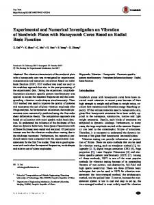
2 Experimental rig The experimental rig (see Fig. I) of the triple physical pendulum consists of the following subsystems:

Q Springer

758

Fig. 1 Experi~nentalrig

pendulum, driving subsystem, and the measurement subsystem. The pendulum consists of a stand that is a symmetrical steel welded construction. The stand consists of a massive frame and two brackets of 1 m long. Each bracket is connected with two blocks that make pendulum affixed to the stand by means of the bearings (the first joint of the pendulum) as well as the driving system and the measuring system. Axial bearings (AXK 1730) and radial bearings (NKI 17/20) are used. The bearings are of high resistance to large loads along with their small dimensions and they provide the elimination of backlash. The joints are made of small aluminum blocks. One of them, that belongs to the first link, functions as a pin of the bearing and the second one serves for fixing a shaft, where the bearing is placed. The aluminum blocks play an important role, namely, they are guides for aluminum rods connecting thejoints. The rods and the blocks make links of the pendulum. These four rods are bored transversely at distances of 10 mm. They are able to move in the bores of these aluminum blocks. Due to this fact, one can ad.just spacing of thejoints i.e., changing the length of the links. The rods are affixed

Q Springer

Nonlinear Dyn (2007) 50:755-766

to the blocks by means of steel threaded pins ended with nuts. The blocks and joining rods are made of aluminum alloy in order to decrease mass of a movable piece of the pendulum. Steel shafts that are elements of the bearing are hollowed axially in order to decrease mass of the pendulum. There are aluminum blocks, which are placed between the joints and the rods that serve for attaching steel weights. The blocks can be displaced along the rods and one can set their position besides changing the number of additional weights. The triple physical pendulum is designed as a system of two symmetrically joined pendulums to eliminate stress caused by torques or forces that do not act in the plane of motion. The pendulum has a module structure, and one can easily disassemble it or change its configuration. Moreover, one can also change parameters such as the mass of the links mi, the position of mass centre of the link ei, the moment of inertia Bi,and the length of the link Ei. The pendulum-driving subsystem consists of two engines of slow alternating currents and optoelectronic commutation. The engine stator consists of 16 aircore coils (the stator coils) and eight optoisolators. The coils are affixed to two round plates of iron "ARMCO" (low-magnetic hysteresis) and are connected in logic circuit, eight sections of four coils (one for each engine). The plates, with the coils on it, are affixed to the earlier described steel blocks and together with the system of eight optoisolators make the engine stator. The part of the optoelectronic system, including eight optoisolators (located on a tape of elastic "Rezotex") is screwed on the circumference of one of the plates. The stator disk possesses eight symmetry axes (22.5") and in order to provide the desired torque, the coils are on a circle of radius 120 mm. The engine stator has been designed in such a way that the current intensity in the windings is linearly dependent on the engine torque. For this purpose, ferromagnetic cores are dropped out because the signal controlling the engine torque varies according to sine function and, in some instants, it takes on values close to zero. Taking heed of this fact, the interaction between the stator cores and the rotor magnets would be very high. It would disturb operation of the engine, thereby making its operation impossible. Engines designed in this manner operates after applying to them nominal voltage. In

Nonlinear Dyn (2007) 50:755-766

our experimental study, we used a square-shape driving torque.

3 LabView environment Analog signals incoming from measuring devices (precise rotational potentiometers) are processed in LabView measurement software. The modular LabView measurement package is presently widely used in industry as complete programmable set of test instruments, which are, in particular, in cooperation with the well-developed block-diagram building software. Dynamic data acquisition (DAQ) is made with the use of the following test instruments: chassis PXI-I01 I, SCXI-1125 module installed in the chassis, the terminal block SCXI-13 13 (high-voltage attenuator), which are in cooperation with the PCI-6052E PC computer's card. The PXI-I011 chassis integrates a highperformance four-slot PXI subsystem with an eight-slot SCXI-subsystem (SCXI-1125 module) to offer a complete solution for signal conditioning and switching applications. The PXI section of the chassis accepts a MXI-3 interface and a wide variety of modules - such as multifunction input/output (MIO), digital input,output (DIO), and computer-based instrument modules. The eight SCXI slots integrate signal conditioning modules into the PXI system. The modules provide analog and digital input conditioning, isolation, and other functions. The SCXI-1125 module is the eight-channel analog input conditioning module with programmable gain and filter settings on each channel. Each channel has 12 programmable gain settings from 1 to 2000 and two programmable filter settings of either 4 Hz or 10 kHz. The National Instruments SCXI- I 125 provide 250-300 V,, of working isolation and low-pass filtering for each analog input channel. This architecture is ideal for amplification and isolation of millivolt sources, volt sources, from 0 to 20 mA, 4 to 20 mA, and thermocouples. It can multiplex these eight channels into a single channel for the DAQ device (SCXI-6052E PC computer 's card), and some other modules can be added to increase channel count. The SCXI-1313 terminal block extends the input range of the previously described module to 300 V,, or 300 VDc, on a per-channel basis programmatically through software commands. The SCXI- 1313 also in-

cludes an onboard temperature sensor for thermocouples cold-junction compensation. The LabView software environment offers the complete library of numerical and mathematical tools, which allow processing of experimental data. Blocks are connected by lines of various colors and pattern in the environment and represent some predefined application procedures (reading and writing to channel inputs and outputs, numerical analysis). The series of measured data are possible to be stored in text files and then showed on any waveforms graphs.

4 Mathematical model of the triple pendulum As a physical model of the real system presented in Section 2, we use the system of three rotationally coupled rigid bodies moving in the vacuum, in the gravitational field of acceleration g, as shown in Fig. 2. The pendulum moves in the plane, and its position is determined by three angles qi (i = 1,2,3). In the joints Oi, the viscous damping with the coefficients ci (i = 1,2, 3) is present. It is assumed that the mass centers of the links lie on the lines including the joints, and one of the principal central inertia axes (zCi)of each link is perpendicular to the pendulum movement plane. The masses of the pendulums are mi, and the moments of inertia with respect to the axes z,i are J,; (i = 1,2,3), respectively.

Fig. 2 Model of the triple physical pendulum

a Springer

760

Nonlinear Dyn (2007)50:755-766

/

*1(t)

&kt)

Model

*2(t) *3(0

IL Fig. 4 The block scheme of the model Fig. 3 The external forcing function

where The first pendulum is externally excited by the square-shape moment of the force fel(t)with the amplitude 9, the angular velocity w , and the initial phase $o, as shown in Fig. 3. The governing equations of the system, shown in the Fig. 2, are

+ e:m + 1:(m2 + 4 , BZ = J z 2 + e;m2 + l;m3, BI = J Z l

I

where

[

C I + C ~

=

-c2

0

-c2

c2

+ c3

-c3

-:3]

c3

M I sin , P(+) = [ M 2 sin $ 2 M3 sin $3

The parameter vector of the pendulum is

a Springer

1

, fdt) =

r"'

,

, )

,

Nonlinear Dyn (2007) 50:755-766

-0.4

-0.2

0

76 1

0.2

0.4

88

90

92

94

t

$1

96 experiment simulation forcing Poincar6 section

98

------

Fig. 5 Final model and real system matching

(f e l ) and three observed outputs ($q, q2,@3), where

by adjusting the parameter vector p, the agreement between the model and real system can be obtained. For more details on the triple pendulum equations and their derivation, see earlier works of the authors [20-221. M3 = I

5 Parameter identification

Note that the paramete.rs of the external forcing ......> .&.,.. F ! . .. . .. (q, w, 4) a.r..e. . rreareu separaiely. rlnally, t n -e .model of the system can be shown as in Fig. 4, with one input \

1,.

-1.

In the mathematical model presented in Section 4, derived from physical laws, the parameter vector p is unknown (forcing parameters are assumed to be known).

Q Springer

762 Fig. 6 Bifurcation diagram for mathematical model

Nonlinear Dyn (2007) 50:755-766 4

0.5

0.7 0.8 0.9 from right t o left from left t o right + solutions used in identification other periodic solutions

0.6

.

f Those parameters should be such that the maximum possible agreement between the model and real system is obtained. By the concept of the mathematical model and real system matching, we understand that the numerical solution ( q I , 7+b2,$9) of the mathematical model behaves in the same way as the corresponding outputs of the real system, with the same inputs and initial conditions for both systems. The following criterion-function of matching the output signals of the real system and model is defined as

where $~i(s.~' = $ f ) ( k ~ t )and $j"'*) = $ , ? ) ( k ~ t )are the model and the real system output series obtained numerically and by measurement, correspondingly, At is sampling period for both model and real system, s is series index, M is number of experimental (numerical) series, i is the pendulum link index, N,Tois the first point index in the sth time series, and N, is the last point index in the sth time series. The forcing signals of the same parameters are led to the model and to the real system, and the same initial conditions are chosen for simulation and experiment for each sth pair of time series. The evaluation of the function F(p) for each new value of p requires s new numerical simulations, with s experimental series once obtained and stored in the computer memory.

B Springer

The model parameter estimation consists in finding the global minimum of the criterion-function (5). For estimating the minimum, the method used is a combination of the simplex method and stochastic shooting near the current value of p. The success of the method depends on the starting point po, which should be the first approximation of the system parameters obtained by the use of some other method. Note that the series used in identification should not include segments with initial conditions sensitivity, i.e., with chaotic behavior, because of problems that can arise with estimating the minimum. It should be noted, that the global minimum finding problem for the function (5) is rather difficult, and we are not certain that the minimum found is really the global one. But, as shown further, the used method can be efficient in finding the model parameter, for which we have a good agreement between the model and the real pendulum. For the parameter estimation we use three different experimental series for three different forcing frequencies f = w/2n = 0.3.0.45, and 0.6 Hz and for the same amplitude q = 2 Nm. Each solution starts from zero initial conditions at t = 0: +Cli(s'" = @?'(o) = 0, (s.0) +Cli(s.O' = +!")(0) = 0, = $,?)(0) = 0, q ; =

-

(s)

qi

$yo)

-

(0) = 0 (i = 1,2,3; s = 1,2,3), with initial phase = & = r.The sampling period is of the forcing At = 0.01 s, and the same time step in the RungeKutta integration of the mathematical model is used. The first and last point indices for each series are Ni0 = 8820 and Ni = 9800 (i = 1,2,3), which corresponds

Nonlinear Dyn (2007) 50:755-766

-0.4

-0.2

0

763

0.2

0.4

288

289

290

291

t

$1

292

293 experiment simulation forcing PoincarB section

294

------

Fig. 7 Model and I.eal system periodic response

to the time interval t E (88.2,98) of each solution taken into account in the evaluation of the function F(p). The following set of parameters, minimizing the criterion-function, have been found

B2=0.1602kgm2, B3=0.01675kgm2,

M2=7.198kgm2/s2, M3=1.158kgm2/s2, (6) \

NI2= 0.1262 kgm2,

cl = 0.06825 kg m2/s,

,

N,, .. = 0.02 1 16 kg - m2, c2 = 0.02216 kg- m2/s, . N23 = 0.02736 kg m2,

c3 = 0.001840 kg m2/s.

The final model and real system matching in the parameter estimation process is presented in Fig. 5. It should be noted that the parameters (6) are optimal in the sense of matching of output model and real system signals rather than in the sense of the real physical values approximation. Especially, the values of the damping coefficients are not rather real. However, as shown

B ' Springer

Nonlinear Dyn (2007) 50:755-766

Fig. 8 Model and real system chaotic response for ,f = 0.73 Hz

in Section 6, the model with parameters (6) fulfils its purpose, and it can be used as a tool for predicting the real pendulum behavior. It can be helpful in quick searching for interesting phenomena in the real system as well as in their explanation.

6 Numerical and experimental results In Fig. 6, two bifurcation diagrams for mathematical model with parameters (6) are shown. Bifurcation di-

a Springer

agrams consist of PoincarC sections of attractors, performed for different forcing frequency values f (bifurcation parameter) and projected on the q3axis. As the PoincarC sections, we have used the sections 4 = 0 (where 4 = o t mod 27r is the phase of the excitation), i.e., periodic sampling of the system state (with period T = 2 n l o = f -')at instances, when the square-shape forcing is at its rising edge. Each section is done for the steady-state behavior of the pendulum, i.e., after omitting some transient motion. In practice, we have waited for 200 forcing periods T, and then the PoincarC section for 100 periods (100 points for each value of f ) have been stored. Then a very small change is introduced in the value of f and new PoincarC section is calculated, using the final state of the previous section, as an initial state, and again omitting IOOT seconds of the transient motion. The vertical resolution of the diagram is the 800 points, i.e., between two successive PoincarC sections' calculations, the change of the frequency value is Af = f(0.9 - 0.3)/800 Hz, where sign depends on whether the bifurcation diagram is performed from left to right or vice versa. The first bifurcation diagram (grey points) is performed from right to left and starts at f = 0.9Hz from zero initial state (then the IOOT second of transient motion is ignored before the first PoincarC section). The second bifurcation diagram (black points), starting from the final state of the first one, is performed from left to right and laid on the first one. In bifurcation diagram depicted in Fig. 6, the periodic solutions used in identification are marked by the use of square symbol, which correspond to the PoincarC sections marked in Fig. 5. Now, we are going to test the model for other forcing frequencies. Figure 7 shows three different periodic solutions obtained from zero initial conditions for forcing frequencies f = 0.5,0.69, and 0.81 Hz, for both the mathematical model and the experiment. The PoincarC point of each periodic solution of the mathematical model is marked by the ball in Figs. 6 and 7. We see rather good agreement between the model and experiment. Note that the experimental solutions (especially, the solution for f = 0.69 Hz and when observing Q3) exhibit some asymmetry, which is not seen when observing the solution of the mathematical model. Bifurcation diagram for the mathematical model exhibits an irregular region for f E (0.700,0.768) Hz. The experiment confirms the existence of this zone for f E (0.695,0.774) Hz. Figure 8 shows an example of

Nonlinear Dyn (2007) 50:755-766

765

Fig. 9 Chaotic attractor exhibited by the model for f = 0.73 Hz Fig. 10 Lyapunov exponents of the chaotic attractor exhibited by the model for f = 0.73 Hz

irregular solution for f = 0.73 Hz obtained both from the experiment and from the model. Firstly, the experimental solution is obtained from zero initial state, as shown in the diagram, after ignoring the transient motion for t > 183 s. Then the numerical solution is computed from the state of the real system at instance t = 183 s. So, we can observe how the solutions diverge quickly due to the initial state sensitivity. Both the experimental and the numerical solutions are irregular with every three links performing full rotations at unpredictable instances. Figure 9 contains three projections of the PoincarC section of the attractor of the mathematical model for f = 0.73 Hz. This section is similar to that described above, for lOOOT seconds of the ignored transient motion and with the 30,000 points stored as shown in diagram. The chaotic character of the presented attractor is confirmed by the Lyapunov exponents computation with results presented in Fig. 10, where three positive exponents are seen. For the computation of the

Lyapunov exponets from the differential equations, the well-known method by Wolf et al. [23] is used. The time of the transient motion ignored is 104S,and computation time is 4 x lo4 s. The period of the GrammSchmidt reorthonormalization is 0.5 s.

7 Concluding remarks In this paper, the experimental rig and the corresponding mathematical model of the triple physical pendulum is presented. The model parameter estimation is performed with three different experimental periodic solutions used. As resulting from the method of estimation used, the model parameters are not optimal in the sense of the best real physical values approximation, but rather in the sense of the best matching of output signals from the model and the real pendulum. From this point of view, the rather artificial values of damping coefficients are not so important (however interesting),

Q Springer

766

but what is important is that the mathematical model with their parameters can be successfully used in prediction of behavior of the real system. The model can be used as a tool for quick searching for various phenomena of nonlinear dynamics exhibited by the real pendulum as well as for their explanation. Some differences between the results from experiment and from numerical solution of the model can arise from two sources. First, the mathematical model may be not sufficiently complex for describing some real physical phenomena in triple pendulum. It especially concerns the damping in thejoints of the real pendulum, where a more complicated phenomena and then a linear damping may be present. Second, the method of global minimum finding for the criterion-function is not perfect. In other words, we never have certainty that we have found the global minimum and not just the local one. Acknowledgements This work has been supported by the Polish Scientific Research Committee (KBN) under the grant no. 4 T07A 03 1 28.

References I. Banning, E.J., van der Weele, J.P.: Mode competition in a system of two parametrically driven pendulums: the Hamiltonian case. Physica A220.485-533 ( 1995) 2. Beckert, S., Schock, U., Schulz, C.D., Weidlich, T., Kaiser, F,: Experiments on the bifurcation behavior of a forced nonlinear pendulum. Phys. Lett. A107.347-350 (1987) 3. Blackburn, J.A., Yang, Z.J., Vik, S.: Experimental study of chaos in a driven pendulum. Physica D26,385-395 (1987) 4. Heng, H., Doerner, R., Hubinger, B., Martienssen, W.: Approaching nonlinear dynamics by studying the motion of a pendulum. I. Observing trajectories in state space. Int. J. Bif. Chaos 4(4), 75 1-760 (1994) 5. Starett, J., Tagg, R.: Control of a chaotic parametrically driven pendulum. Phys. Rev. Lett. 74, 1974-1977 (1995) 6. Piiroinen, D.T., Virgin. L.N., Champneys, A.R.: Chaos and period-adding: experimental and numerical verification of the grazing bifurcation. J. Nonlinear Sci. 14,384-404 (2004) 7. Zhu, Q., Ishitobi, M.: Experimental study ofchaos in a driven triple pendulum. J. Sound Vib. 227(1), 230-238 (1999)

Q Springer

Nonlinear Dyn (2007) 50:755-766 8. Awtar, S., King, N., Allen,T., Bang, I., Hogan, M.,Skidmore, D., Craig, K.: Inverted pendulum systems: rotary and armdriven - a mechatronic system design case study. Mechatronics 12,357-370 (2002) 9. Yoshida, K., Sato, K.: Characterization of reverse rotation in chaotic responseof mechanical pendulum. Int. J. Non-Linear Mech. 33(5), 8 19-828 ( 1998) 10. Galan, J., Fraser, W.B., Acheson. D.J., Champneys, A.R.: The parametrically excited upside-down rod: an elastic jointed pendulum model. J. Sound Vib. 280, 359-377 (2005) I I . Acheson, D.J.: A pendulum theorem. Proc. R. Soc. London A443,239-245 ( 1993) 12. Braun, M.: On some properties of the multiple pendulum. Arch. Appl. Mech. 72,899-910 (2003) 13. BolteZar, M., Hammond, J.K.: Experimental study of the vibrational behavior of a coupled non-linear mechanical system. Mech. Syst. Signal Process. 13(3), 375-394 (1999) 14. Furata,T.,Tawara,T.,Okumura, Y.,Shimizu, M.,Tomiyama, K.: Design and construction of a series of compact humanoid robots and development of biped walk control strategies. Robotics Autonom. Syst. 37.81-100 (2001) 15. Selles, R.W., Bussmann, J.B.J., Wagenaar, R.C., Stam, H.J.: Comparing predictive validity of four ballistic swing phase models of human walking. J. Biomech. 34, 1171-1 177 (200 1) 16. Donelan, J.M., Kram, R., Kuo, A.D.: Simultaneous positive and negative external mechanical work in human walking. J. Biomech. 35, 1 17-1 24 (2002) 17. Miyashita, T., Ishiguro, H.: Human-like behavior generation based on involuntary motions for humanoid robots. Robotics Autonom. Syst. 48,203-2 12 (2004) 18. Awrejcewicz, J., Kudra, G.: The piston-connecting rodcrankshaft system as a triple physical pendulum with impacts. Int. J. Bif. Chaos 15(7), 2207-2226 (2005) 19. Sygniewicz, J.: Modeling of Cooperation of the Piston with Piston Rings and Barrel (in Polish). Sci. Bull., 6 151149,Technical University of t 6 d t (1991) 20. Kudra, G.: Analysis of Bifurcations and Chaos in Triple Physical Pendulum with Impacts (in Polish). PhD thesis, Technical University of t 6 d i (2002) 21. Awrejcewicz, J., Kudra, G., Lamarque, C.-H.: Dynamics investigation of three coupled rods with a horizontal barrier. Spec. Issue Meccanica 38(6), 687-698 (2003) 22. Awrejcewicz, J., Kudra, G., Lamarque, C.-H.: Investigation of triple pendulum with impacts using fundamental solution matrices. Int. J. Bif. Chaos 14(12), 4191-4213 (2004) 23. Wolf, A.. Swift, J.B., Swinney, H.L., Vastano, J.A.: Determining Lyapunov exponents from a time series. Physica D16,285-3 17 (1985)