MATEC Web of Conferences 145, 03003 (2018) https://doi.org/10.1051/matecconf/201814503003 NCTAM 2017
Experimental and numerical investigation of plasma parameters in the magnetosheath Polya Dobreva1,*, Monio Kartalev1, Olga Nitcheva1, Natalia Borodkova2, and Georgy Zastenker 2 1Institute of Mechanics, Bulgarian Academy of Sciences, Acad. G. Bonchev Str., block 4, Sofia, Bulgaria 2Space Research Institute, Russian Academy of Sciences, Profsoyuznaya Str., 84/32, 117997 Moscow, Russia
Abstract. We investigate the behaviour of the plasma parameters in the magnetosheath in a case when Interball-1 satellite stayed in the magnetosheath, crossing the tail magnetopause. In our analysis we apply the numerical magnetosheath-magnetosphere model as a theoretical tool. The bow shock and the magnetopause are self-consistently determined in the process of the solution. The flow in the magnetosheath is governed by the Euler equations of compressible ideal gas. The magnetic field in the magnetosphere is calculated by a variant of the Tsyganenko model, modified to account for an asymmetric magnetopause. Also, the magnetopause currents in Tsyganenko model are replaced by numericaly calulated ones. Measurements from WIND spacecraft are used as a solar wind monitor. The results demonstrate a good agreement between the model-calculated and measured values of the parameters under investigation.
1 Introduction The Earth magnetosheath is a transitional region between the bow shock and the magnetopause in which the solar plasma is heated, decelerated and compressed. It plays a crucial role in solar-terrestrial relations, because the solar wind energy is transmitted through it and propagates to the magnetosphere and ionosphere. That is why it is important to understand how characteristics of the interplanetary medium are modified in this transitional region. The picture is further complicated by the presence of a variety of structures and waves within a wide frequency, inherent to the magnetosheath itself. The first gas-dynamic description of the magnetosheath was given in the pioneer model of Spreiter [1]. The model presents two-dimensional picture of flow properties in the magnetosheath for given input data, which are the solar wind Mach number, polytropic index and a predetermined magnetopause position. Later, the model was further developed to calculate the magnetic field in the magnetosheath [2]. Although the model takes into account the solar wind variations in some extend, it was not adapted to practical purposes and has some serious shortcomings. For example, it does not allow for the north-south and *
Corresponding author:
[email protected]
© The Authors, published by EDP Sciences. This is an open access article distributed under the terms of the Creative Commons Attribution License 4.0 (http://creativecommons.org/licenses/by/4.0/).
MATEC Web of Conferences 145, 03003 (2018) https://doi.org/10.1051/matecconf/201814503003 NCTAM 2017
dawn-dusk asymmetries in bow shock and magnetopause geometries and does not take into account the indentations around the cusp area at the magnetopause [3]. The numerical magnetosheath-magnetosphere model provides a three-dimensional description of the plasma flow in the magnetosheath, based on the gas-dynamics. The magnetosheath boundaries are self-consistently determined in the process of solution. The model takes into account the cusp indentations at the magnetopause, the dawn-dusk and north-south displacement at the bow sock (BS) and magnetopause (MP) positions in the tail. Moreover, the model is relatively simple, it does not require extensive computing resources and is executed on a personal computer. The model was already applied in interpretation of Interball-1 measurements [4, 5, 6]. The main parameter under investigation was the ion flux, which values were compared in several events, when the satellite crossed the magnetosheath. The aim of this paper is to investigate the behaviour of the plasma parameters in a case when the satellite stayed in the magnetosheath, crossing the magnetopause only. Parameters to be considered are the ion flux and velocity along the Interball-1 orbit. On January 16-18, 1997 Interball-1 was in the northern tail at about -15 RE (Earth radii) moving southward and it stayed in the magnetosheath for about 32 hours, several times crossing the magnetopause. Short description of the model is presented in Section 2. The necessary solar wind data are described in Section 3.1, the magnetosheath ones – in Section 3.2, and the results of the comparison are given in Section 4.
2 Brief description magnetosphere model
of
the
numerical
magnetosheath-
The numerical magnetosheath-magnetosphere model is based on the modular approach, that allows separate model to be applied in the each of the two interconnected regions. The relation between these separate regions is established by the conditions, imposed at the boundaries. The magnetosheath description is based on the gas-dynamic approximation, as we assume that the flow is compressible ideal gas, governed by the Euler’s equations. As a result of the simulation the velocity, density and temperature in the magnetosheath are obtained and as a consequence we calculate the gasdynamic pressure and the Mach number distributions. The numerical scheme [7], which is a variant of the method of characteristics, is applied in solving the system of equations. The magnetic field in the magnetosphere is sum of several contributions: filed of the Earth’s dipole, the field, due to the tail, Birkeland and ring currents and the field of the Chapman-Ferraro currents. Our model allows for the calculation of the magnetopause currents, confining the magnetic field into the magnetosphere with an arbitrary geometry. The field of the external sources – the ring, Birkeland and tail currents, is calculated by a variant of Tsyganenko model – T95 [8] or T01 [9]. The Tsyganenko model is modified as the shape of its magnetopause is not used, instead, it is to be found in the process of simulation. Besides, the magnetopause currents, related to that particular form of the MP are replaced by ones, calculated via the finite element method. The penetration of magnetic field across the magnetopause is not allowed and B n=0. The interaction between these two models is achieved through the boundary conditions. The Rankine-Hugoniot relations, expressing the conservation of mass, energy and momentum are imposed at the magnetopause and the bow shock. At the points of the magnetopause these conditions are reduced to the equation of pressure balance. The method applied here is capable of describing the real size and geometry of the bow shock and the magnetopause, including the cusp indentations at the magnetopause, the north-sought and
2
MATEC Web of Conferences 145, 03003 (2018) https://doi.org/10.1051/matecconf/201814503003 NCTAM 2017
dawn-dusk asymmetries in the tail magnetosheath boundaries. Moreover, there is no need to rescale the trajectory of the satellite passage through magnetosheath in order to coincide with the model boundaries. Input data, needed for the calculations are: the density, velocity and temperature of the solar wind; By and Bz components of the IMF (Interplanetary Magnetic Field); Dst index (based on the Kyoto Web page); the dipole tilt angle; polytropic index γ. Description of the magnetosheath properties is based on the single fluid approach, as the density and velocity are that of the ions, but the temperature is a sum of the ion and electron temperatures. A more detailed description of the numerical model, used here, can be found in some previous papers [4, 10, 11]
3 Satellite measurements, used in the study 3.1 Solar wind data On January 16-18, 1997 WIND spacecraft [12] was situated in the solar wind at about 130136 RE from the Earth. Here, we use WIND data as a solar wind monitor. The propagation time of the solar wind from WIND to Interball-1 is in the range 48~55 min. Fig. 1 and Fig. 2 present the input plasma and magnetic field data. The proton number density Fig. 1a) gradually increases from 8 sm-3 at the beginning of the interval, reaches its peak of about 28 sm-3 at 20:50 UT January 17 then decreases to 12 sm-3 after 04:00 UT January 18. The velocity varies in the range -300~-350 km/s – Fig. 1b). The temperature rises after 00:00 UT on January 18, as electron temperature increases twice and proton temperature - more than twice – Fig. 1c).
Fig. 1. Input plasma parameters, measured by the WIND spacecraft on January 16-18, 1997: a) proton number density; b) Vx component of the velocity; c) proton temperature Ti (gray) and electron temperature Te (green). Data are not shifted in time.
The variations of the IMF, based on the WIND spacecraft are presented in Fig. 2. The input magnetic field is northward during the interval 20:00 UT January 16 to 08:00 UT January 17, then it is duskward and mainly southward during the interval [08:00-20:00 UT] on January 17. After that, it changes its direction several times and is strongly dawnward at a four-hour interval [01:00-05:00 UT] January 18.
3
MATEC Web of Conferences 145, 03003 (2018) https://doi.org/10.1051/matecconf/201814503003 NCTAM 2017
The data of solar wind density, velocity and electron temperature are based on WIND/SWE (Solar Wind Experiment) instrument [13], the proton temperature - on WIND/3DP (3D Plasma Analyzer) – [14]. The IMF data are measured by WIND/MFI (Magnetic Field Investigator) device [15]. The time resolution is 1.5 min for the density and velocity, 12 sec for the electron temperature, 3s for the proton temperature and 1 min for the magnetic field. However, for our purposes the temperature data are averaged over 1 min intervals.
Fig. 2. a), b), c) Bx, By and Bz components of the Interplanetary Magnetic Field measured by the WIND spacecraft on January 16-18, 1997. Data are plotted in GSE (Geocentric Solar Ecliptic) system of coordinates and are not shifted in time.
3.2 Magnetosheath data
Fig. 3. Interball-1 trajectory from 19:00 UT January 16 to 08:00 UT January 18, 1997. The projections shown are on (X, Y, Z=0) and (X=-14, Y, Z) GSE coordinate planes (the distances are in Earth radii). The inner dashed curve represents the magnetopause of Shue 97 [20] calculated with parameters - dynamic pressure Pd= 2 nPa and IMF Bz=0 nT. The outer dashed curve is the shape of the bow shock, calculated by our model for the given Shue form, mentioned above. The point denotes the beginning of the interval.
4
MATEC Web of Conferences 145, 03003 (2018) https://doi.org/10.1051/matecconf/201814503003 NCTAM 2017
Interball-1 is a high apogee satellite, part of the Interball Project [16], which primary objective was to study the solar–terrestrial relations. It was in operation from August 1995 until October 2000 and moved in strictly elliptical orbit with an apogee of about 195000 km and a perigee in the range 500-10000 km – [17]. Measurements of the ion flux are based on the Omnidirectional plasma sensor VDP - [18]. The device consisted of four integral Faraday cups - C1, C2, C3 and C4. The C1 sensor was oriented along the principal axis of the satellite, which deviated up to 10º from the Sun-Earth line, thus collecting the flux coming from the Sun. Directions of the other three sensors –C2, C3 and C4 were perpendicular to this axis (see the device description [18]). The time resolution of the Interball-1 data was 1s, but for our purposes the flux measurements were averaged over 1 min intervals. The velocity data are based on the CORALL device (more details are given in [19]) and have a time resolution of 2 min. During February – September of each year the satellite completed an orbit in four days period, meanwhile crossing the magnetosheath twice.
Fig. 4. Ion flux, measured onboard Interball-1 (blue) and onboard WIND (gray) satellites on January 16-18, 1997. Here the MP labels depict the moments of Interball-1 crossings of the magnetopause. WIND data are shifted appropriately.
Interball-1 orbit during the interval 19:00 UT January 16 to 08:00 UT on January 18 is presented in Fig. 3. The satellite is in the dusk sector at about -13~-15 RE in the tail, moved from north to south, as during the second half of the interval it is close to the equatorial GSE plane. In the interval, we observe multiple magnetopause crossings and the satellite stayed in the magnetosheath for about 32 hours without crossing the bow shock. The ion flux and ion velocity (both in x direction), conducted onboard Interball-1 satellite, are given in Fig. 4. The corresponding solar wind values, shifted appropriately, are also added in the plot. The satellite first entered the magnetosheath at 20:30 UT January 16 and finally left at 4:53 UT January 18. The flux drop and the corresponding velocity peaks, observed during the intervals [20:47-21:05 UT] on January 16, [03:00-03:13 UT] and [04:13-04:40 UT] on January 17 are connected with the satellite’s re-entering in the magnetosphere. During the interval [04:13-04:53 UT] January 18 the device encountered both magnetosheath and magnetospheric plasma. The peak of the flux is associated with the solar wind flux increase, and before 10:00 UT January 17 and after 01:00 UT January 18 the flux in the magnetosheath is lower that the solar wind one.
5
MATEC Web of Conferences 145, 03003 (2018) https://doi.org/10.1051/matecconf/201814503003 NCTAM 2017
4 Model results In the present paper we apply the comparison algorithm, that we have used in earlier papers considering Inteball-1 measurements - [4, 5, 6]. We divide the whole interval into five subintervals [20:30 UT January 16 - 03:00 UT January 17], [03:00-09:00 UT January 17], [09:00-16:00 UT January 17], [16:00 UT January 17 - 01:00 UT January 18], [01:00-04:53 UT January 18]. Then we run the model with sets of input parameters, corresponding to each interval. The parameters at the first and last intervals correspond to the time moments near the magnetopause crossings. The parameters of the solar wind and interplanetary medium applied in the simulations are given in Table 1, the ratio of specific heats is γ=2. Table 1. Input data, used in the simulations: dynamic pressure P d (in nPa), Mach number, By and Bz GSE components (in nT), Dst index and dipole tilt angle (in degrees). UT
Pd
M
By
Bz
Dst
tilt
21:05(16/01)
1.26
6.43
1.5
-0.5
-12
-15.6º
06:00(17/01)
1.47
6.33
0.6
2.0
-1
-30.3º
12:00(17/01)
2.08
6.44
2.5
-1.8
6
-17.4º
21:50(17/01)
4.69
6.56
1.3
-3.0
1
-17.2º
04:10(18/01)
1.98
5.06
-4.5
-1.0
-5
-30.0º
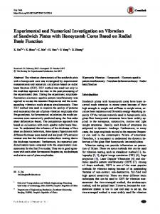
The magnetosheath geometry and velocity distribution in the plane that passes through the satellite location at the moment of MP crossing at 04:10 UT (January 18) are presented in Fig. 5a). The tick black curve is the projection of the spacecraft orbit. The satellite registered moment of crossing (denoted by the outer yellow point) agrees well with the model calculated magnetopause. a
b
Fig. 5. Left a): Distribution of the model-calculated Vx component of the ion velocity, corresponding to the moment of the MP crossing at 04:10 UT January 18. Right b): Distribution of the modelcalculated ion flux (in X direction), based on the moment of 21:50 UT January 17. The black line on both panels depicts the satellite trajectory during [12:00 UT January 16 - 12:00 UT January 18]. The yellow points on the left denote the spacecraft location at the moments of the two MP crossings 20:30 UT January 16 (inner point) and 4:53 UT January 18 (outer point). The plasma parameters are shown in non dimensional units.
The magnetosheath geometry and the ion flux distribution in the plane that passes through the satellite location at the moment 21:50 UT (January 17) are presented in Fig. 5b). The satellite trajectory during the interval is depicted by a black line. Note that around
6
MATEC Web of Conferences 145, 03003 (2018) https://doi.org/10.1051/matecconf/201814503003 NCTAM 2017
21:50 UT January 17 the solar wind density increased to about 28 sm -3 that is more than four times higher than the average solar wind density of 6 sm -3. The increase of the solar wind density - Fig. 1a), and respectively the dynamic pressure, resulted in magnetopause compression. Thus, the satellite remained deeper in the magnetosheath - Fig. 5b). The behaviours of the ion flux and velocity, according to Interball-1 data and to the model calculations are shown in Fig. 6. The model flux most significantly differs from the measured one at the interval close to the MP crossing [02:00- 4:53 UT January 19]. It is lower than the satellite-registered flux at the interval [11:00 -22:00 UT January 17] (17% on average) and is slightly higher at the interval [20:30 UT January 16 – 10:00 UT January 17]. One can see that the flux increases from 2 (x10 8 sm3s-1) at the beginning of the interval to about 10 (x108 sm-3s-1) at 22:00 UT January 17. This increase of the flux is related to the rise of the solar wind flux (added by a thin gray line), which is well represented by the numerical model. The experimental and model-calculated Vx velocities are plotted in Fig. 6 (bottom). The magnetosheath velocity is about 68-75% from the solar wind one – Fig. 5a), Fig. 6 (bottom). As the trajectory is close to the equatorial GSM (Geocentric Solar Magnetospheric) plane the flow has a strong Vx component - about 200 km/s, as expected. The model velocity differs from the experimental one most in the interval [20:30- 24:00 UT January 16] where the difference is about 20%. In the whole interval the result of the simulations is in good agreement with the measurements, the difference is about 11% on average as the model values been higher (in absolute value) – Fig. 6 (bottom).
Fig. 6. Comparison between the Interball-1 (blue) and the model-calculated (green) ion flux (top panel) and ion velocity (bottom). The thin grey line represents the solar wind values, shifted accordingly. The MP labels denote the moment of magnetopause crossings, registered by the satellite.
5 Summary We investigated the behaviour of two parameters in the magnetosheath – the ion flux and velocity. We compared the model estimates with the data, based on satellite’s measurements. The satellite stayed for a long time in the magnetosheath, remaining close to the magnetopause. The model adequately represents the velocity values and the strong variation of the flux in the magnetosheath. The paper is supported by the Bulgarian National Council “Scientific Research” under Project DMU 03/88.
7
MATEC Web of Conferences 145, 03003 (2018) https://doi.org/10.1051/matecconf/201814503003 NCTAM 2017
References 1. 2. 3. 4. 5. 6. 7. 8. 9. 10. 11. 12. 13. 14. 15. 16. 17. 18. 19. 20.
J.R. Spreiter, A.L. Summers, A.Y. Alksne, Planet. Space. Sci. 14, 223-253, (1966) J.R. Spreiter, S.S. Stahara, J. Geophys. Res. 85, 6769-6777, (1980) J.R. Spreiter, S.S. Stahara, Adv. Sp. Res. 7, 5-19, (1994) P.S. Dobreva, M.D. Kartalev, M.D. Shevyrev, G.N. Zastenker, Planet. Sp. Sci. 53, 117125, (2005) G.N. Zastenker, M.D. Kartalev, P.S. Dobreva, N.N. Shevyrev, A. Koval, Cosm. Res. 46(6), 469-483, (2008) P.S. Dobreva, M.D. Kartalev, N.L. Borodkova, G.N. Zastenker, Adv. Sp. Res. 58, 188195, (2016) A.S. Magomedov, K.M. Holodov, Grid Characteristic Numerical Method, Nauka, Moscow, (1988) N.A. Tsyganenko, J. Geophys. Res. 100, 5599-5612, (1995) N.A. Tsyganenko, J. Geophys. Res. 107(A8), 10.1029/2001JA000219, (2002) P.S. Dobreva, M.D. Kartalev, D. Koitchev, V.I. Keremidarska, M. Kaschiev, Adv. Sp. Res. 41, 1279-1285, (2008) M. Kartalev, P. Dobreva, E. Amata, M. Dryer, S. Savin, J. Atm. Sol. Terr. Phys. 70(24), 627-636, (2008) M.H. Acuna, K.W. Ogilvie, D.N. Baker, S.A. Curtis, D.H. Fairfield, W.H. Mish, Space Sci. Rev. 71, 521, (1995) K.W. Ogilvie, D.J. Chornay, R.J. Fritzenreiter et al., Space Sci. Rev. 71, 41-54, (1995) R.P. Lin, K.A. Anderson, S. Ashford et al., Space Sci. Rev. 71(1-4), 125-153, (1995) R.P. Lepping, M.H. Acuna, L.F. Burlaga et al., Space Sci. Rev. 71, 207-218, (1995) A.A. Galeev, Yu.I. Galperin, L.M. Zelenyi, Cosm. Res. 34(4), 339-362, (1996) R.S. Kremnev, A.I. Smirnov, S.S. Gorkin, Cosm. Res. 34(4), 363–370, (1996) J. Safrankova, G. Zastenker, Z. Nemecek, et al., Ann. Geophys. 15, 562-569 (1997) Yu.I. Yermolaev, A.O. Fedorov, O.L. Vaisberg, Ann. Geophys. 15(5), 533-541, (1997) J.-H. Shue, J.K. Chao, H.C. Fu et al., J. Geophys. Res. 102(A5), 9497-9511, (1997)
8