Mechanics and Mechanical Engineering Vol. 15, No. 3 (2011) 297–307 c Technical University of Lodz ⃝
Experimental Validation of Numerical Model within a Flow Configuration of the Model Kaplan Turbine
Zbigniew Krzemianowski The Szewalski Institute of Fluid–Flow Machinery, Gda´ nsk Polish Academy of Sciences
[email protected] Marzena Banaszek Krzysztof Tesch Gda´ nsk Univeristy of Technology
[email protected] [email protected] Received (10 August 2011) Revised (15 September 2011) Accepted (23 September 2011)
This paper investigates validations of flow within a model Kaplan turbine. This includes comparison of various turbulence models and their influence on torque and power generated by the turbine. Numerical were compared with experimental data. Keywords: Turbomachinery, fluid mechanics, hydraulic turbines
1.
Introduction
The primary aim of the present investigation was the numerical analysis of an existing model Kaplan turbine with adjustable stator and rotor. The turbine is mounted on a test stand at the Mechanical Engineering Department of Gdansk University of Technology, and has been thoroughly experimentally investigated, resulting in the identification of optimum setting combination of the stator and rotor. This experimentally determined efficiency-optimal work point has been taken as the basis of numerical modeling. Computational Fluid Dynamics (CFD) is well established in the analysis of turbomachinery flows for over 20 years. The literature, however, enumerates computational results using commercial solvers with arbitrarily chosen turbulence models, typically selected on the basis of user experience. It should be noted that there is no single, universally applicable turbulence model; its appropriate selection for a specific computational case rests on expert judgement. As the authors had at their
Krzemianowski, Z., Banaszek, M., Tesch, K.
298
disposal accurate and comprehensive experimental results, it was decided to deliberately carry out computation employing a broad range of turbulence models with variants. The following models were employed: one–dimensional Spalart–Allmaras, two dimensional k–ε and k–ω. For the k–ε model the analysis has been carried out for assorted variants of the model, distinguished by various methods of boundary layer modeling (Standard, Non–Equilibrium, Enhanced) and by different viscosity models (algebraic or differential). Altogether twelve numerical variants were used, and the varying results were checked against the experimental standard. Numerical analysis was carried out using the Ansys Fluent solver, a popular choice for many technical applications. On this basis conclusions were drawn with regard to the pattern of pressure losses along the turbine flowpath, as modeled by the several turbulence model variants.
2.
Flowpath geometry
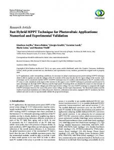
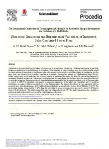
Fig.1 shows schematically the existing turbine test stand. The flow cycle takes place as follows: The headwater tank (2) is topped up by pump (1) drawing water from channels running below floor level. The upper head is maintained at the constant level by an overflow weir returning excess water to the supply channels. From the tank the flow passes through a duct containing in succession: a vaned bend (3), the structural pre–stator, the stator proper (4), the rotor (5) and the draft tube (6), from where it passes into the metering channel. In the channel are flow stabilizers (7) and a rectangular (Hansen type) flow–metering weir (8). Past the weir, the flow is returned to the supply channels. The flowpath traversed–pump, tank, turbine, channel, pump–runs in a closed cycle recycling its water. The laboratory setup incorporates a vertical in–pipe turbine. It is supplied through a vaned offset inlet (3). The inlet contains a cascade of fixed vanes redirecting and organizing flow. In the vertical section of the duct, above the turbine, is a ring of streamlined shaft–support struts constituting the pre–stator. The stator proper (4) is located below in a section of the duct bounded by segments of spherical surfaces around the hub and the periphery, facilitating rotation of the adjustable guide vanes. Vane adjustment axes are inclined at 75˚ with respect to turbine axis, while the hub and rim faces of the vanes are shaped to mate with the spherical hub and duct lining. Vane shafts pass through duct wall and are connected via cranks to a governor ring wrapping around the duct. The vanes can be rotated to a position where they completely close off duct clearance, serving as a cut–off valve. Turbine rotor (5) of characteristic diameter D = 0.265 m has blades that can be adjusted while the turbine is off–line. The vertical shaft of the rotor is supported by two bearings, one of which is radial and occupies the hub of the guide ring, while the other carries radial and axial loads and is located outside the duct, above the offset inlet. The top extremity of the shaft is coupled to a DC generator (10), which serves also as the brake. The computational model of flowpath geometry is shown and schematically dimensioned in Fig. 2. The computational flowpath comprised five sections:
Experimental Validation of Numerical ...
1
2
3
13
10 12
299
15 16
14
9
7
4 11 5 6
1 2 3 4 5 6 7 8
pump upper water reservoir pipe bend guide rotor draft tube straighteners Hansen's rectangular weir
9 10 11 12 13 14 15 16
float direct current generator ring clutch manometric level indicator needle water level gauge probes piezometers
Figure 1 Experimental stand for model turbine investigation
140
Figure 2 Computational geometry of the analyzed flowpath
8
Krzemianowski, Z., Banaszek, M., Tesch, K.
300
SECTION 1: Offset inlet, including five vanes redirecting horizontal inflow from the tank in the downward direction. The turbine shaft shroud passes through the row of vanes and exits through the upper wall. SECTION 2: Six stationary vertical guide vanes comprising the prestator (shaft support ring). The pre–stator is necessary for structural reasons, but serves the additional function of stabilizing and aligning the flow above the inlet to stator proper. The vanes are streamlined and aligned with the axial direction. SECTION 3: Twelve adjustable vanes of the stator proper, serving to generate angular momentum in the stream prior to entering the rotor. In the computational model the vanes were set at 20o with respect to the transverse cross– sectional plane, in order to duplicate the experimentally–determined conditions for optimal–efficiency turbine performance. SECTION 4: Six rotor blades. In the computational model the blades were set at 16˚ with respect to the transverse cross–sectional plane, for the reason mentioned above. SECTION 5: Axially–symmetrical draft tube. 3.
Computational model of the flowpath
The computational mesh was prepared in two stages. At the first stage, the mesh for the rotor and for the stators was prepared using the Numeca AutoGrid tool. After transferring the fragmentary mesh to Ansys Gambit, the mesh was completed by meshing the draft tube and the offset inlet. The completed meshed geometry was divided into five subsections. The subsections serve as stage points for comparison of pressure drops. The complete mesh consists of some 7 million elements. The mesh consists entirely of hexahedral elements, and was structured to achieve values of the dimensionless wall parameter (Y+ ) in the range 1 to 3. Inflow into the computational flowpath was set as normal to the inlet surface. 4.
Numerical computation of flow
The computation has been carried out with the aid of the Fluent solver included in the Ansys 12.1 package, with the additional assumption of stationary flow and using a second order discretization scheme. Carried out to double precision, the computation required on the order of 20000 iterations. As noted in the introduction, the computations were carried out using several turbulence models for comparison. Three fundamental turbulence models were used: one–dimensional Spalart–Allmaras, two dimensional k–ε and two–dimensional k–ω. The multitude of available options for the k–ε models prompted an additional in– depth investigation, the variants differentiated by various methods of boundary layer modeling (Standard, Non–Equilibrium, Enhanced) which were expected to introduce noticeable variation in computation results. Furthermore, within the k– ε RNG variant, the algebraic and differential model of viscosity were separately investigated. In total, the following computational variants have been modeled: 1. Spalart–Allmaras; 2. k–ε Standard Enhanced;
Experimental Validation of Numerical ...
301
3. k–ε RNG Standard; 4. k–ε RNG Standard – Differential Viscosity Model; 5. k–ε RNG Non–Equilibrium; 6. k–ε RNG Non–Equilibrium – Differential Viscosity Model; 7. k–ε RNG Enhanced; 8. k–ε RNG Enhanced – Differential Viscosity Model; 9. k–ε Realizable Standard; 10. k–ε Realizable Non–Equilibrium; 11. k–ε Realizable Enhanced; 12. k–ω SST. Boundary conditions were chosen to match the conditions extant during experimental testing. Specifically, the following boundary conditions were set: Inlet. At the inlet plane the absolute pressure was set as pt BC = 26726 Pa, which corresponds to a head of 2.725 m with respect to the outlet plane; this was taken directly from laboratory measurement. The inflow was set as normal to the inlet plane. Outlet. At the outlet from the draft tube the static pressure was set as ps = 0 Pa. The gauge level of pressure is irrelevant for incompressible flow as modeled, as long as pressures at various points within the flow are gauged with respect to the same reference, here set at zero for convenience. Wall. The non–slip condition of zero relative velocity was set at walls. Interfaces. Four interfaces were defined within the flowpath: between the inlet duct and the pre-stator, between the pre–stator and the stator, between the stator and the rotor, and between the rotor and the draft tube. The interfaces are surfaces where non–matching meshes abut; the values of parameters at non–coincident nodes at the interface are interpolated by the solver. Turbulence parameters (identical for all variants used): Inlet: turbulence intensity: 3.525 %, hydraulic diameter: 0.4 m Outlet: turbulence intensity: 3.771 %, hydraulic diameter: 0.685 m turbulence intensity was derived from Reynolds number according to the formula I= 16Re −1/8 [%] General: rotation speed of rotor: 650 RPM, water density: 999.7 kg/m3 5.
Numerical computation results and comparison with experimental values
The results of computation are presented below. Some tables include experimental values for comparison, which were obtained on the described test stand at Gdansk University of Technology. The experimental data included: shaft torque (and consequently shaft power output), mass flow rate measured at the rectangular weir, and the efficiency computed on that basis.
Krzemianowski, Z., Banaszek, M., Tesch, K.
302
Table 1 Numerical and experimental result: torque, mass flow rate, efficiency
Lp.
1. 2. 3. 4.
5. 6.
7. 8.
9. 10.
11. 12.
Experiment and turbulence models Experiment Spalart– Allmaras k-ε Standard Enhanced k-ε RNG Standard k-ε RNG Standard - Differential Viscosity Model k-ε RNG NonEquilibrium k-ε RNG NonEquilibrium Differential Viscosity Model k-ε RNG Enhanced k-ε RNG Enhanced - Differential Viscosity Model k-ε Realizable Standard k-ε Realizable NonEquilibrium k-ε Realizable Enhanced k-ω SST
Torque (Power) (ω= 68.068 rad/s)
Mass flow rate
Efficiency
M (P) [Nm (W)] 25.900 (1763.0) 25.709 (1750.0)
m [kg/s] 74.302 74.140
η [%] 88.73 88.48
24.308 (1654.6)
73.327
84.62
24.450 (1664.3)
74.058
84.33
25.347 (1725.3)
73.781
87.86
23.427 (1594.6)
74.172
80.66
25.581 (1741.2)
74.836
87.36
25.156 (1712.3)
73.783
87.15
25.094 (1708.1)
73.745
86.99
24.976 (1700.1)
74.215
85.85
23.988 (1632.8)
74.130
82.55
25.783 (1755.0)
74.201
88.66
25.780 (1754.8)
74.353
88.51
Tab. 1 summarizes the key quantities calculated for the several computational variants and measured in the experiment, specifically the torque, power, mass flow rate and efficiency. Tab. 2 compares relative and absolute variation from the experimental values for the mass flow rates computed for the investigated turbulence models, Tab. 3 compares results and actual data for the torque.
Experimental Validation of Numerical ...
303
Table 2 Comparison of relative and absolute variation from the experimental values for the mass flow rates computed for the investigated turbulence models
Lp.
1. 2. 3. 4.
5. 6.
7. 8.
9. 10.
11. 12.
Experiment and turbulence models Experiment Spalart– Allmaras k-ε Standard Enhanced k-ε RNG Standard k-ε RNG Standard - Differential Viscosity Model k-ε RNG NonEquilibrium k-ε RNG NonEquilibrium Differential Viscosity Model k-ε RNG Enhanced k-ε RNG Enhanced - Differential Viscosity Model k-ε Realizable Standard k-ε Realizable NonEquilibrium k-ε Realizable Enhanced k-ω SST
Mass flow rate
Relative deviation
Absolute deviation
m [kg/s] 74.302 74.140
[%] -0.22
[kg/s] -0.162
73.327
-1.33
-0.975
74.058
-0.33
-0.243
73.781
-0.71
-0.520
74.172
-0.17
-0.130
74.836
0.71
0.534
73.783
-0.70
-0.518
73.745
-0.76
-0.557
74.215
-0.12
-0.087
74.130
-0.23
-0.171
74.201
-0.14
-0.101
74.353
0.07
0.051
The efficiency listed above was computed as: η=
P Mω = ρgHQ gHm
(1)
where: M [Nm] – numerically obtained total shaft torque, comprising pressure torque Mpress and viscosity torque Mvisc (the latter, acting on the blading, hub, and cowl,
Krzemianowski, Z., Banaszek, M., Tesch, K.
304
Table 3 Comparison of computed torques, their constituents, and their relative and absolute variation from the experimental values, for the investigated turbulence models
Lp
1. 2.
3. 4.
5.
6.
7. 8.
9.
10.
11.
12.
Experiment and turbulence models
Experiment SpalartAllmaras k-ε Standard Enhanced k-ε RNG Standard k-ε RNG Standard Differential Viscosity Model k-εgNG NonEquilibrium k-ε RNG NonEquilibrium - Differential Viscosity Model k-ε RNG Enhanced k-ε RNG Enhanced Differential Viscosity Model k-ε Realizable Standard k-ε Realizable NonEquilibrium k-ε Realizable Enhanced k-ω SST
Pressure Viscosity Torque Relative torque torque deviation of torque M press M visc M [%] [Nm] [Nm] [Nm] 25.900 26.699 -0.990 25.709 -0.74
Absolute deviation of torque [Nm]
25.412
-1.104
24.308
-6.55
-1.592
26.179
-1.728
24.451
-5.93
-1.449
25.921
-0.574
25.347
-2.18
-0.553
26.071
-2.644
23.427
-10.56
-2.473
26.547
-0.966
25.580
-1.25
-0.320
26.170
-1.014
25.156
-2.96
-0.744
26.104
-1.009
25.094
-3.21
-0.806
26.664
-1.687
24.976
-3.70
-0.924
26.670
-2.682
23.988
-7.97
-1.912
26.818
-1.035
25.783
-0.45
-0.117
26.775
-0.994
25.780
-0.47
-0.120
-0.191
Experimental Validation of Numerical ...
305
Table 4 Comparison of hydrodynamic forces and their numerically obtained constituents for the investigated turbulence models
Lp.
Turbulence models
1.
SpalartAllmaras k-ε Standard Enhanced k-ε RNG Standard k-ε RNG Standard - Differential Viscosity Model k-εgNG NonEquilibrium k-ε RNG NonEquilibrium Differential Viscosity Model k-ε RNG Enhanced k-ε RNG Enhanced - Differential Viscosity Model k-ε Realizable Standard k-ε Realizable NonEquilibrium k-ε Realizable Enhanced k-ω SST
2. 3. 4.
5. 6.
7. 8.
9. 10.
11. 12.
Pressure force
Viscous force
Total force
T press [N] 783.24
T visc [N] 3.29
T [N] 786.53
766.25
4.11
770.36
757.83
5.31
763.13
761.94
1.59
763.53
757.31
8.26
765.56
787.20
2.86
790.06
747.74
3.25
750.99
745.98
3.21
749.18
780.75
5.55
786.30
777.96
8.91
786.87
772.96
3.58
776.53
784.98
3.21
788.18
is opposed to Mpress , resulting in the reduction of total torque) M = Mpress + Mvisc ω [rad/s] – angular velocity of the rotor (ω = 68.068 rad/s); P [W] – shaft output power; ρ [kg/m3 ] – density of water; g [m/s2 ] – acceleration of gravity; Q [m3 /s] – volume flow rate ;
(2)
Krzemianowski, Z., Banaszek, M., Tesch, K.
306
H [m] – net turbine head; Tab. 4. presents the hydrodynamic force T for the various turbulence models. This has also been split into components due to pressure Tpress and to viscosity Tvisc , as it has been done for the torque. It may be interesting to note that the viscous term of this force has the same sign as the pressure term, so unlike the corresponding moments the forces are summed. 6.
Conclusions
The computation has brought to light significant and not unexpected discrepancies between the obtained values for flow efficiency yielded by the disparate methods of turbulence modeling. The highest value, and the closest to experimental validation, has been provided by the k–ε Realizable Enhanced model (88.66 %), closely followed by the results of the k–ω SST model (88.51 %) and the Spalart–Allmaras model (88.48 %), the experimental reference value being 88.73 %. The remaining models yielded still lower results for the efficiency. Four of these, specifically: k–ε RNG Standard–Differential Viscosity Model (87.86 %), k–ε RNG Non-EquilibriumDifferential Viscosity Model (87.36 %), k–ε RNG Enhanced (87.15 %), and k–ε RNG Enhanced–Differential Viscosity Model (86.99 %) have achieved accuracy within 2%, while the remaining models have underestimated efficiency more significantly. The worst performer in this regard was the k–ε RNG Non-Equilibrium model (80.66 %). All the predicted efficiency estimates are lower than actual experimental results, even though superficially it would seem the opposite ought to hold. Some inaccuracy in experimental measurement of flow rate (using the rectangular weir) cannot be ruled out; and yet the disparity in numerical and experimental results is only marginally due to different flow rates, which cannot account for the whole of the observed effect. Analyzing the differences in individual quantities impacting efficiency leads to the conclusion that the largest disparity is due to differences in computed and measured torque on the turbine shaft. All the computed variants yielded values of torque significantly lower than the value actually measured (25.9 Nm). The difference ranges from as little as 0.45 % (k–ε Realizable Enhanced) to a whopping 10.56 % (k–ε RNG Non–Equilibrium). The discrepancies between predicted and measured values of mass flow rate resulted in a similar, but smaller effect, with the error in numerical values ranging from –1.33 % do 0.76 % with respect to the measured value of 74.302 kg/s. Overall, the computations in Fluent appear to predict flow rates quite accurately. The selection of a suitable turbulence model is of paramount importance with regard to accuracy of expected results. Choosing the wrong model may result in glaring divergence from realizable results. This is particularly important when experimental verification is not feasible. Under such circumstances, the choice must be guided by operator experience, parameters of the generated mesh (appropriate Y + ), and the boundary (initial) conditions being set. Application of three variants of the differential viscosity model improves the efficiency prediction (k–ε RNG Standard, k–ε RNG Non–Equilibrium) or maintains it at the same level (k–ε RNG Enhanced). It is consequently suggested that the DVM be used in conjunction with the k–ε RNG model.
Experimental Validation of Numerical ...
307
References [1] Banaszek, M., and Tesch, K.: On Some Method of Flow Configuration Optimisation in Kaplan Turbine, Computer Methods in Mechanics, Warsaw, Poland, 2011. [2] Krzemianowski Z., and Banaszek, M.: Numerical computation of the flowpath through a model Kaplan turbine with axial inflow, IMP PAN, nr 48/2011, 2011. [3] Krzemianowski Z., and Banaszek, M.: Numerical computation of the flowpath through a model Kaplan turbine with with offset inflow, and comparison with experimental results, IMP PAN, nr 77/2011,2011. [4] Banaszek, M.: Theoretical and experimental analysis of flow through a stage of a model hydraulic turbine, PhD thesis (supervisor: prof. dr hab. in. R. Puzyrewski), Gda´ nsk University of Technology, Gda´ nsk, 2002.