AVEC 10
Experimental Validation of Terrain-Aware Rollover Prediction for Ground Vehicles Using the Zero-Moment Point Method Sittikorn Lapapong, Alexander A. Brown, and Sean N. Brennan∗ Department of Mechanical and Nuclear Engineering, The Pennsylvania State University 318 Leonhard Building, University Park, PA 16802 USA Phone: +1-814-863-2430 Fax: +1-814-865-9693 E-mail:
[email protected],
[email protected], and
[email protected] Rollover accidents are one of the leading causes of death in highway accidents due to their very high fatality rate. A key challenge in preventing rollover via chassis control is that the prediction of the onset of rollover can be quite difficult, especially in the presence of terrain features typical of roadway environments. These road features include superelevation of the road (e.g. road bank), the median slope, and the shoulder down-slope. This work develops a vehicle rollover prediction algorithm that is based on a kinematic analysis of vehicle motion, a method that allows explicit inclusion of terrain effects. The solution approach utilizes the concept of zero-moment point (ZMP) that is typically applied to walking robot dynamics. This concept is introduced in terms of a lower-order model of vehicle roll dynamics to measure the vehicle rollover propensity, and the resulting ZMP prediction allows a direct measure of a vehicle rollover threat index. Field experimental results show the effectiveness of the proposed algorithm under different driver excitations. Topics / Vehicle Rollover Control, Vehicle Dynamics, Active and Passive Safety Systems ∗
Corresponding author
1. INTRODUCTION According to the U.S. Department of Health and Human Services [1], motor vehicle accidents are the leading cause of death in the United States when causes of death by disease are not included. In 2007, automobile crashes claimed 41,059 lives, and 2,491,000 people were injured in 6,024,000 police-reported motor vehicle traffic crashes [2]. These reports indicate that 8,940 out of 41,059 lives were lost in rollover accidents, indicating that vehicle rollover is one of the major causes of death for highway accidents. To reduce deaths due to the vehicle rollover accidents, it is very important to improve vehicle safety, especially roll stability of the vehicle. In both academic and industrial institutions, there have been many efforts to measure and predict vehicle rollover propensity. The efforts are primarily to construct rollover threat metrics that are useful for predicting rollover onset, thus providing a measurement for indicating a rollover-prone vehicle. Further, the metrics are used for alerting the driver during a rollover-prone situation, or even for active chassis control to prevent rollover. These metrics can be generally categorized as follows: static or steady-state rollover metrics, dynamic rollover metrics, energy-based rollover metrics, rollover metrics
based on thresholds of vehicle states or combinations of the vehicle states, and rollover metrics based on forces acting on tires or body moments generated by those forces. Examples of static or steady-state rollover metrics include the Static Stability Factor (SSF) [3], the Side-Pull Ratio (SPR) [3], the TiltTable Ratio (TTR) [3], the centrifuge test [3], the Bickerstaff’s rollover index [4], and related rollover thresholds for a suspended vehicle model [5]. Issues with these types of metrics are that they do not include dynamics of a vehicle or road conditions into consideration, and they do not provide a realtime warning capability. These issues can be addressed by introducing the dynamics of the vehicle to a rollover-metric formulation process or using vehicle states at a particular driving situation to anticipate rollover events. The dynamic rollover metrics are based on the Newton’s second law of motion, for instance, the Dynamic Stability Index (DSI) [5]. Energy-based metrics are another efforts to employ the vehicle states to measure vehicle rollover propensity. Examples of the energy-based metrics include the Critical Sliding Velocity (CSV) [6] and the Rollover Prevention Energy Reserve (RPER) [5] Often, vehicle states, for example roll angle, roll rate, lateral acceleration, etc. or combinations thereof, are used to detect vehicle rollover either directly or
AVEC 10 with ad-hoc metrics. Examples of rollover metrics using vehicle states include Wielenga [7], Carlson and Gerdes [8], and Yoon et al. [9]. Similarly, rollover metrics can be based on situation-dependent tire forces and/or moments such as the Load Transfer Ratio (LTR) [10] and the Stability Moment (SM) [11]. Another example using moments would be the study by Cameron [12] who predicted a minimum steering angle that caused vehicle rollover by determining the existence of a slide-before-roll condition. Finally, one can extend the prediction of vehicle states, forces, or moments into the future to anticipate rollover events, for example, the work of Chen and Peng who proposed Time-To-Rollover (TTR) metric [13]. For a rollover metric to be useful, the prediction of rollover behavior needs to be accurate, particularly predicting the onset of rollover such as tire lift. Since, referring to a National Highway Traffic Safety Administration (NHTSA)’s report [14], the majority of all rollover accidents are due to either on-road tripped rollover or off-road rollover in which terrain plays a significant role, this research differentiates from previous studies to develop a more accurate tire-lift prediction by including the effects of terrain. There are quite a few rollover metrics (load transfer ratio and stability moment) that concern the influences of the terrain; however, the implementation of these metrics is still an issue, since the LTR and SM are based on terrain/tire interaction forces that are not trivial to obtain. Additionally, once wheel liftoff occurs, the numerical values of these metrics saturate (be either -1 or 1) due to the ways that the metrics are defined. Under this circumstance, the metrics are deprived of the sense of the severity of the encountering rollover situation. To deal with these matters, we adopt a method used by walking robots called the Zero-Moment Point (ZMP), a concept introduced in Section 2 of the paper. Section 3 discusses an application of the ZMP as a vehicle rollover threat index, which is followed by field experimental results in Section 4 to show fidelity of the proposed algorithm. Conclusions then summarize the main contributions of this paper.
zero. Here, the tipping moments are defined as the component of the moment that is tangential to the supporting surface [19]. For a kinematic chain to be dynamically stable, the location of the ZMP must lie within the support polygon. However, if the support polygon is not large enough to encompass the location of the ZMP to balance the action of external moments, this can result in overturn of the kinematic chain [20]. To be more strict, this zero-moment point must be within the support polygon of the mechanisms; otherwise, this point does not physically exist. If the location of the ZMP is calculated, and it is outside the support polygon, that point is considered as a fictitious ZMP (FZMP) [20]. To be more precise, it should be noted that the term ZMP is not a perfectly exact expression, because the normal component of the moment generated by the inertia forces acting on the biped is not necessarily zero. Hence, we should keep in mind that the term ZMP abridges the exact expression “zero tipping moment point” [19].
2. ZERO-MOMENT POINT (ZMP)
where mi is the mass of the ith body, Ii is the inertia tensor of the ith body, ~ai is the linear acceleration of the ith body, ω ~ i is the angular velocity of the ith body, p~i = ~ri − ~rzmp , ~ri is the position vector of the center of gravity (CG) of the ith body, ~rzmp is the position vector of the ZMP, and ~g is gravitational ~ A = [0 0 MA ]T , the point A beacceleration. If M z comes a zero-moment point.
The concept of zero-moment point (ZMP) was developed and introduced by Vukobratovic in 1968 [15]. This concept has been very useful and widely used in bipedal robotics research. Biped robotics scientists have applied the concept to preserve robots’ dynamic balance during walking, or, in other words, to maintain stability of the robots, preventing the robots from overturning. There are hundreds of biped walking robots implemented with this algorithm, for instance, Honda’s humanoid robots [16]. Moreover, many researchers used the ZMP as a stability constraint for mobile manipulators to prevent the overturn of the mobile manipulators due to their own dynamics [17, 18]. By definition, the zero-moment point is the point on the ground where the tipping moment acting on the biped, due to gravity and inertia forces, equals
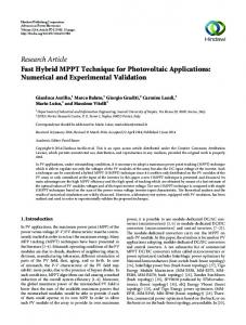
Fig. 1: Two-link kinematic chain Considering a kinematic chain in Fig. 1 and using general equations of motion [21, 22, 23] and D’Alembert’s principle [24], the moment equation about point A in Fig. 1 induced by inertial forces and gravity is: MA = p ~1 × m1~aG1 + I1 ω ~˙ 1 + ω ~ 1 × I1 ω ~1 − p ~1 × m1~g (1) ˙ +p ~2 × m2~aG + I2 ω ~2 + ω ~ 2 × I2 ω ~2 − p ~2 × m2~g 2
3. APPLICATION OF ZERO-MOMENT POINT AS VEHICLE ROLLOVER THREAT INDEX In this section, the concept of the ZMP is applied as an indicator to predict vehicle rollover. The convention of the coordinates [25] and the sequence of coordinate rotations [26] used in this section are defined by the Society of Automotive Engineers (SAE).
AVEC 10 3.1 Application to Rigid Vehicle Model In this section, the concept of the ZMP is applied to a vehicle modeled as a rigid body shown in Fig. 2.
Fig. 2: Rigid vehicle model
Table 1: Nomenclature and vehicle properties for rigid vehicle model Symbol Definition Value Unit m mass of vehicle 3321 kg a distance from 1.89 m CG to front axle b distance from 1.46 m CG to rear axle h height of CG 1.22 m T track width 1.62 m Ixx,yy,zz mass moment of inertia about x-axis 2030 kg·m2 y-axis 7751 kg·m2 z-axis 7862 kg·m2 Ixz,yz product mass 0 kg·m2 moment of inertia φr roll angle vsa rad φt roll angle of rad terrain θ pitch angle vs rad p roll rate vs rad/s q pitch rate vs rad/s r yaw rate vs rad/s aG CG’s accelerationb vs m/s2 a b
(a)
(b)
Fig. 3: Rigid vehicle model on terrain. (a) φr ≥ φt (b) φr < φt The nomenclature used in derivations of this section is defined in Table 1, Fig. 2, and Fig. 3. In Fig. 2, the coordinates oxyz are fixed with the vehicle at the center of gravity of the vehicle (point G). Point Q is a zero-moment point located by ~rzmp and is always physically on the ground. To calculate the location of the zero-moment point, we assume that the vehicle is symmetrical in the xzplane (Ixy = 0), and the vehicle is free to move in any directions. Considering Fig. 3, the location of the ZMP may be expressed as: ~ rzmp = xzmp~i + yzmp~j · ¸ T + h + |tan(φr − φt )| − yzmp tan(φr − φt ) ~k 2
vs = vehicle state acquired through sensors instrumented on a vehicle. Subscripts x, y, and z indicate accelerations in x-, y-, and z- directions.
direction (about the x-axis), allowing the unsprung mass and sprung mass have the same angular velocities and accelerations except in the roll direction. The sprung mass is supported by a roll spring (Kφ ) and roll damper (Dφ ) that act as the vehicle’s suspensions. In the figure, point G is the location of
(2)
By using Eq. 1, the location of the ZMP can be expressed as: yzmp = {mT |tan(φr − φt )| [g cos(θ) sin(φr ) − aGy] + 2 [− Ixx p˙ + Ixz pq + Iyz q
2
+ (Iyy − Izz )qr − Iyz r
2
+ Ixz r˙ + mgh cos(θ) sin(φr ) − mhaGy}
/ {2m [g cos(θ) cos(φt ) sec(φr − φt ) − aGz − aGy tan(φr − φt )]} (3)
Since the main focus of this work is to predict vehicle rollover, only the expression of yzmp is presented for brevity. 3.2 Application to Vehicle Roll Model A vehicle is modeled as illustrated in Fig. 4. The vehicle consists of two parts: unsprung mass and sprung mass. Both masses are linked together at the point called a roll center (point R). The roll center allows the sprung mass to rotate only in the roll
Fig. 4: Vehicle roll model the whole vehicle’s center of gravity (CG). Point Gu and point Gs are the centers of gravity of unsprung mass’s and sprung mass’s, respectively. The sprung mass’s CG is located by ~rs , which is (c + d)~i + (hs − hr ) sin(φ)~j+[hu + hr (cos(φ) − 1) − hs cos(φ)] ~k. The notations used in this section are defined in Table 2, Fig. 4, and Fig. 5. The coordinates oxyz are attached with the unsprung mass’s center of gravity whose distance is d measured from the vehicle’s CG. Point Q in Fig. 4 is the zero-moment point, which is located by ~rzmp .
AVEC 10
(a)
(b)
Fig. 5: Vehicle roll model on terrain. (a) φu ≥ φt (b) φu < φt In the same fashion as in Section 3.1, the position vector of the ZMP may be expressed as: ~ rzmp = xzmp~i + yzmp~j · ¸ (4) T + hu + |tan(φu − φt )| + yzmp tan(φu − φt ) ~k 2
The location of the ZMP can be solved by using Eq. 1, which is: yzmp = {T |tan(φt − φu )| [ms (−g cos(θ) sin(φu ) + asy ) + mu (−g cos(θ) sin(φu ) + auy )] − 2 [(Iyzs + Iyzu )q
2
+ (Iyys + Iyyu − Izzs − Izzu )qr ! Ã φ + φu − (Iyzs + Iyzu )r + (Ixzs + Ixzu )r˙ + ms hr (−2g cos(θ) cos 2 Ã ! Ã ! φ 2 φ sin − 2asy sin + asz sin(φ)) + ms hs (g cos(θ) sin(φ + φu ) 2 2 2
− asy cos(φ) − asz sin(φ)) + mu hu g cos(θ) sin(φu ) − mu hu auy + Ixzs ps q + Ixzu pu q − Ixxs p˙ s − Ixxu p˙ u]} / {2 [ms (g cos(θ) cos(φt ) sec(φt − φu ) − asz + asy tan(φt − φu )) + mu (g cos(θ) cos(φt ) sec(φt − φu ) − auz + auy tan(φt − φu ))]} (5)
Again, since the focus of this paper is primarily on lateral rollover, the expression of xzmp is ignored. However, the solutions of xzmp for both rigid vehicle model and vehicle roll model are provided in [27]. 4. EXPERIMENT SETUP From simulation results [27], one can see that the simulation results seem to be very promising. However, to truly validate the merit of the zero-moment point method, field experiments are needed. The test vehicle is a robotically-driven 1989 GMC 2500 pickup truck shown in Fig. 6. The truck is instrumented
Fig. 6: Test truck
Table 2: Nomenclature and vehicle properties for vehicle roll model Symbol Definition Value Unit ms sprung mass 3022 kg mu unsprung mass 299 kg a distance from total 1.89 m CG to front axle b distance from total 1.46 m CG to rear axle c distance from total 0.05 m CG to ms ’s CG d distance from total 0.15 m CG to mu ’s CG hs height of ms ’s CG 1.26 m hu height of mu ’s CG 0.35 m hr height of roll center 0.5 m T track width 1.62 m Ixx,yy,zz x-axis, y-axis, #b kg·m2 z-axis mass moment of inertiaa Ixz,yz product mass 0 kg·m2 a moment of inertia φs roll angle of ms vsc rad φu roll angle of mu vs rad φ φs − φu rad φt roll angle of rad terrain θ pitch angle vs rad p roll ratea vs rad/s q pitch rate vs rad/s as acceleration of ms ’s CGd vs m/s2 d au acceleration of mu ’s CG vs m/s2 a b c d
Subscripts s and u indicate the properties of sprung mass and unsprung mass of the vehilce roll model, respectively. Ixxs =1665, Iyys =6913, Izzs =6879, Ixxu =145, Iyyu =802, Izzu =947 vs = vehicle state acquired through sensors instrumented on a vehicle. Subscripts x, y, and z indicate accelerations in x-, y-, and zdirections.
truck to acquire states of unsprung mass. To detect wheel liftoff, infrared range sensors are mounted on the vehicle’s wheel hubs to determine distance to the ground. In addition, string potentiometers are installed on the vehicle’s suspension to measure wheel travel, redundantly serving the same purpose. Furthermore, suspension travel is used to calculate roll angle of unsprung mass. Approximately 850 kilograms of extra weight is added to the truck’s bed, making the truck more rollover-prone. Outriggers are bolted to the front and rear bumpers to prevent the truck from catastrophic rollover. The truck was excited under two maneuvers, Toyota’s J-turn and double-lane change, on a relatively-flat road at speed of 10 m/s. The tests were conducted at the Thomas D. Larson Pennsylvania Transportation Institute’s test track. 5. RESULTS
with a Global Positioning System (GPS) and an Inertial Measurement Unit (IMU) to collect vehicle states that are used to calculate the location of ZMP. Moreover, another IMU is attached to the rear axle of the
In this section, the proposed rollover prediction algorithms from both the rigid vehicle model (Eq. 3) and the vehicle roll model (Eq. 5) are implemented.
Percentage of suspension travel (%)
150
Two−wheel lift
One−wheel lift
One−wheel lift
100 50 0 −50
Front left Rear left Front right Rear right
−100 −150 0
2
4
6
8
10
12
14
16
18
Time (s)
1 0.5 Track width
Displacement of yzmp (m)
1.5
0 −0.5 yzmp of rigid vehicle model
−1 −1.5
yzmp of roll model 0
2
4
6
8
10
12
14
16
18
Time (s)
Fig. 7: Percentage of suspension travel and displacements of yzmp of vehicle during Toyota’s J-turn on flat road at 10 m/s, causing wheel liftoff. A few observations can be seen from the results. First, the displacements of yzmp from both the rigid vehicle model and the roll model predict vehicle rollover quite well. The displacements of yzmp estimated from both models are almost on top of each other and are very hard to distinguish. However, when zooming in the wheel-lift regions, one can see that the displacement of yzmp estimated from the rigid vehicle model (Eq. 3) is a little bit more conservative than the one obtained from the roll model (Eq. 5). This may happen since the roll model is more realistic than the rigid vehicle model, making the behaviors of the roll model closer to a real vehicle than those of the rigid vehicle model. The second observation is
One−wheel lift One−wheel lift
100
Two−wheel lift One−wheel lift
50 0 −50
Front left Rear left Front right Rear right
−100 −150 0
2
4
6
8
10
12
14
16
18
12
14
16
18
20
Time (s)
1.5 1 0.5
Track width
Displacement of yzmp (m)
The algorithms are tested with the test truck described in Section 4. String potentiometers are mounted on the truck’s suspensions to determine when wheel liftoff has occurred. Truck properties (e.g. mass, mass moments of inertia, etc.) used to calculate the locations of yzmp of the rigid vehicle model and vehicle roll model are respectively listed in Table 1 and Table 2. Most of physical properties of the unladen truck are estimated by empirical formulae provided in [28] and [29], except mass moments of inertia of the unsprung mass that are taken from those of a 1987 Ford E150 van [30]. Fig. 7 shows the percentage of suspension travel and displacements of yzmp calculated from Eqs. 3 and 5 of the vehicle that was excited by a Toyota’s J-turn on a flat road at speed of 10 m/s, leading to the wheel liftoff. Fig. 8 illustrates the results during the double-lane-change maneuver on the flat road that induced the wheel liftoff. 100 percent of suspension travel means that the truck’s suspension is fully extended, or, in other words, that wheel liftoff is happening. The shaded regions in the figures indicate the regions where wheel liftoff has occurred. The cyan areas mark the regions in which only one wheel is lifted, usually either side of the front wheels. The yellow areas are the two-wheel-lift regions.
Percentage of suspension travel (%)
AVEC 10
0 −0.5 yzmp of rigid vehicle model
−1 −1.5
yzmp of roll model 0
2
4
6
8
10
Time (s)
Fig. 8: Percentage of suspension travel and displacements of yzmp of vehicle during double-lane change on flat road at 10 m/s, causing wheel liftoff. that the displacement of yzmp during wheel liftoff is a relatively flat straight line. Since there is no external force applied to the vehicle, the only place that reaction forces can physically act after the wheel liftoff is on the edge of the vehicle, allowing the vehicle to rock itself on its wheels due to the effects of its own momentum. Thus we see that the ZMP method also saturates as do other metrics (i.e. load transfer ratio and stability moment), but this saturation is due to physics and not due to the way that the metric is defined. 6. CONCLUSIONS The concept of the ZMP has been introduced and an application of the ZMP point as a rollover threat index for ground vehicles has been presented. From the experimental results, one can see that the ZMP is a valid indicator to measure the vehicle rollover propensity. Both rigid vehicle model and roll model predict vehicle rollover well. Further, the roll model, as expected, predicts the vehicle rollover more precisely than the rigid vehicle model does due to more realistic assumptions of the roll model. This work is still ongoing. More experimental results on different road profile at various speeds are necessary to firmly show the effectiveness of the proposed algorithm, and a rollover mitigation control based on the ZMP will be designed to improve vehicle roll stability. 7. ACKNOWLEDGEMENTS The authors would like to thank the financial support from the Thomas D. Larson Pennsylvania Transportation Institute. Further, the author Sittikorn Lapapong gratefully acknowledges the financial support from the Ministry of Science and Technology, the Royal Thai Government.
20
AVEC 10 REFERENCES [1] M. Heron, D. L. Hoyert, S. L. Murphy, J. Xu, K. D. Kochanek, and B. Tejada-Vera, “Deaths: Final data for 2006,” National Vital Statistics Reports, vol. 57, no. 14. [2] NHTSA’s National Center for Statistics and Analysis, “Traffic safety facts: 2007 data,” DOT HS 810 993. [3] Transportation Research Board, The National Highway Traffic and Safety Administration’s Rating System for Rollover Resistance. Washington, D.C.: National Academy Press, 2002. [4] D. J. Bickerstaff, “The handling properties of light trucks,” SAE Tech. Paper Series, no. 760710, 1976. [5] R. V. Dukkipati, J. Pang, M. S. Qatu, G. Sheng, and Z. Shuguang, Road Vehicle Dynamics. Warrendale, PA: Society of Automotive Engineers, Inc., 2008. [6] I. S. Jones, “Road accident studies with particular reference to the handling and stability characteristics of cars,” Ph.D. dissertation, University College London, 1973. [7] T. J. Wielenga, “A method for reducing on-road rollovers–anti-rollover braking,” SAE Tech. Paper Series, no. 1999-01-0123, 1999. [8] C. R. Carlson and J. C. Gerdes, “Optimal rollover prevention with steer by wire and differential braking,” in Proc. 2003 ASME IMECE, vol. 72 DSC, no. 1, Washington, DC, Nov. 2003, pp. 345–354. [9] J. Yoon, D. Kim, and K. Yi, “Design of a rollover index-based vehicle stability control scheme,” Veh. Syst. Dyn., vol. 45, no. 5, pp. 459–475, 2007. [10] R. D. Ervin and Y. Guy, “The influence of weights and dimensions on the stability and control of heavy-duty trucks in canada Volume I,” The University of Michigan Transportation Institute, Ann Arbor, MI, Tech. Rep. UMTRI-8635/I, July 1986. [11] S. C. Peters and K. Iagnemma, “Stability measurement of high-speed vehicles,” Veh. Syst. Dyn., vol. 47, no. 6, pp. 701–720, 2008. [12] J. T. Cameron, “Vehicle dynamic modeling for the prediction and prevention of vehicle rollover,” Master’s thesis, The Pennsylvania State University, 2005. [13] B.-C. Chen and H. Peng, “Differential-brakingbased rollover prevention for sport utility vehicle with human-in-the-loop,” Veh. Syst. Dyn., vol. 36, no. 4-5, pp. 359–389, 2001. [14] National Highway Traffic Safety Administration, “An experimental examination of selected maneuvers that may induce on-road, untripped light vehicle rollover–phase I-A of NHTSA’s 1997-1998 vehicle rollover research program,” DOT HS 809 357. [15] M. Vukobratovi´c and D. Juriˇci´c, “Contribution to the synthesis of biped gait,” in Proc. IFAC Symp. Technical and Biological Problem on Control, Erevan, USSR, 1968.
[16] K. Hirai, M. Hirose, Y. Haikawa, and T. Takenaka, “The development of honda humanoid robot,” in Proc. IEEE Int. Conf. on Robotics and Automation, vol. 2, Leuven, Belgium, May 1998, pp. 1321–1326. [17] S. Sugano, Q. Huang, and I. Kato, “Stability criteria in controlling mobile robotic systems,” in Proc. IEEE Int. Conf. on Intelligent Robots and Systems, Tokyo, Japan, July 1993, pp. 832– 838. [18] Q. Huang and S. Sugano, “Manipulator motion planning for stabilizing a mobile-manipulator,” in Proc. IEEE Int. Conf. on Intelligent Robots and Systems, vol. 3, Pittsburgh, PA, Aug. 1995, pp. 467–472. [19] P. Sardain and G. Bessonnet, “Forces acting on a biped robot. center of pressure–zero moment point,” IEEE Trans. Syst., Man, Cybern. A, vol. 34, no. 5, pp. 630–637, Sept. 2004. [20] M. Vukobratovi´c and B. Borovic, “Zero-moment point–thirty five years of its life,” Int. J. Humanoid Robotics, vol. 1, no. 1, pp. 157–173, Mar. 2004. Singapore: [21] H. Baruh, Analytical Dynamics. McGraw-Hill Book Co., 1999. [22] A. Dasgupta and Y. Nakamura, “Making feasible walking motion of humanoid robots from human motion capture data,” in Proc. IEEE Int. Conf. on Robotics and Automation, vol. 2, Detroit, MI, May 1999, pp. 1044–1049. [23] J. Kim and W. K. Chung, “Real-time zero moment point compensation method using null motion for mobile manipulators,” Advanced Robotics, vol. 20, no. 5, pp. 581–593, 2006. [24] J. L. Meriam and L. G. Kraige, Engineering Mechanics: Dynamics, 4th ed. New York, NY: John Wiley & Sons, Inc., 1997. [25] W. F. Milliken and D. L. Milliken, Race Car Vehicle Dynamics. Warrendale, PA: Society of Automotive Engineers, Inc., 1995. [26] “Vehicle dynamics terminology–SAE J670e,” Society of Automotive Engineering, Inc., Warrendale, PA, Tech. Rep., Jul 1976. [27] S. Lapapong and S. Brennan, “Terrain-aware rollover prediction for ground vehicles using the zero-moment point method,” in Proc. Amer. Control Conf., Baltimore, MD, June 2010. [28] National Highway Traffic Safety Administration, “Vehicle dynamic stability and rollover,” DOT HS 807 956. [29] P. M. Riede, Jr., R. L. Leffert, and W. A. Cobb, “Typical vehicle parameters for dynamics studies revised for the 1980s,” SAE Tech. Paper Series, no. 840561, 1984. [30] G. J. Heydinger, “Improved simulation and validation of road vehicle handling dynamics,” Ph.D. dissertation, The Ohio State University, 1990.