Radio Science, Volume ???, Number , Pages 1–8,
Experimental Verification of RFI Mitigation with a Focal Plane Array Feed James R. Nagel1 Lockheed Martin, Inc. Vandenberg Air Force Base, CA 93437
Karl F. Warnick,2 Brian D. Jeffs3 Department of Electrical and Computer Engineering Brigham Young University 459 Clyde Building, Provo, UT 84602
J. Richard Fisher,4 and Richard Bradley5 National Radio Astronomy Observatory6 Charlottesville, VA 22903
We demonstrate the use of spatial filtering algorithms for radio frequency interference (RFI) mitigation in conjunction with a focal plane array of electrically small elements. The array consists of a seven-element hexagonal arrangement of thickened dipole antennas with 1600 MHz designed center frequency backed by a circular ground plane at the focal plane of a 3 m parabolic reflector. Rooftop-mounted signal sources were used to simulate a weak signal of interest at boresight and a strong, broadband interferer in the reflector sidelobes. Using an adaptive beamformer, the amplitude of the interfering signal was reduced sufficiently to recover the signal of interest. For an interference to noise ratio of 15 dB as measured at the center array element, the interferer was suppressed to the level of the fluctuations of the 10-second integrated noise floor (the minimum detectable signal level was interference-limited and no longer decreases after 10 s integration). Similar cancellation performance was demonstrated for a nonstationary interferer moving at an angular velocity of 0.1◦ per second. Pattern rumble due to beamformer adaptation was observed and quantified. For a moving RFI source, the degree of pattern rumble was found to be unacceptably large in terms of its effects on the maximum stable integration time and receiver sensitivity. An array feed with more elements together with specialized signal processing algorithms designed to suppress pattern rumble will likely be required in order to use adaptive spatial filtering for astronomical observations.
1. Introduction
approaches to RFI mitigation have received considerable attention. In this paper, we present experimental verification of RFI mitigation for a reflector antenna with a focal plane array (FPA) feed in conjunction with adaptive beamforming algorithms. FPAs have been used for decades for such applications as multi-beam synthesis or compensation for reflector surface aberrations [Blank and Imbriale, 1988]. More recent efforts include the Netherlands Foundation for Research in Astronomy (ASTRON) FARADAY array of broadband Vivaldi antennas for multi-beam synthesis [Ivashina et al., 2004]. The Parkes radio telescope has demonstrated a 13 element waveguide feed FPA [Staveley-Smith et al., 1996] which has been used operationally for the H1 Parkes all-sky survey (HIPASS) [Koribalski, 2002]. FPAs similar to the Parkes array employ electrically large elements individually matched to the reflector surface. Although electronic beamforming can be employed, each element provides a high gain, high spillover effi-
As radio telescopes increase in sensitivity, science applications move away from traditional protected spectral line bands, and man-made radio sources grow in number, techniques for radio frequency interference (RFI) mitigation become increasingly important. Time blanking, adaptive cancellation, spatial filtering, as well as other 1
[email protected] [email protected] 3
[email protected] 4
[email protected] 5
[email protected] 6 The NRAO is operated for the National Science Foundation (NSF) by Associated Universities, Inc. (AUI) under a cooperative agreement. 2
Copyright 2007 by the American Geophysical Union. 0048-6604/07/$11.00
1
Pre-production draft. Copyright 2007, American Geophysical Union
2
NAGEL, ET AL.: ARRAY FEED EXPERIMENTS
ciency beam without beamforming. To achieve greater control over beam patterns, feed arrays of electrically small elements have also been considered for use in radio astronomy applications [Fisher and Bradley, 2000]. Numerical simulations have been used to determine the sensitivity and noise performance of seven and nineteenelement dipole arrays in the presence of RFI [Hansen et al., 2005]. This paper reports an experimental verification of RFI mitigation using a seven-element array of thickened dipoles over a ground plane, at the focal plane of a threemeter parabolic reflector. A weak signal of interest (SOI) obscured by a broadband simulated RFI source was recovered using conventional adaptive beamformer algorithms for both stationary and nonstationary interferers. We also characterize the performance of adaptive cancellation algorithms as a function of interferer power level, and quantify the degree of undesirable pattern rumble due to adaptive beamforming in the case of a nonstationary RFI source.
tion coefficient less than -10 dB with a system impedance of 50 Ω. Each element feed port was attached to a low-noise amplifier and receiver with 105 K noise temperature for each channel. The receiver was a two-stage mixer with a intermediate bandwidth centered at 4 MHz to allow for analog to digital conversion. Sampled data was streamed to a disk array. Complex basebanding and signal processing were performed in post-processing.
2. Array Feed Description
The time average output power relative to a 1 Ω load for M samples is
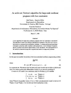
The prototype array feed, depicted in Fig. 1, consisted of seven dipole antennas arranged in a hexagonal grid over a ground-plane backing. The array elements were designed for a center frequency of 1600 MHz (λ = 18.75 cm). The element spacing was fixed at 0.6 λ (11.25 cm), which is small enough to fully sample the focal plane field distribution [Fisher and Bradley, 1999]. The ground plane of the array was formed by 1.5 mm copper-clad laminate.
Figure 1. Seven element array feed geometry.
The array elements were balun-fed thickened dipoles placed at a distance of 0.25 λ above the ground plane. The arms of the dipole were constructed from 6.0 mm copper tubing, with a radius-to-wavelength ratio of a/λ = 0.016. This provided a 30% bandwidth based on an input reflec-
3. Signal Processing The system architecture consists of seven antenna elements connected to parallel receiver chains, followed by signal processing to form a linear combination of the receiver outputs. If the complex voltage samples at the output of each receiver chain at time step n are arranged into a column vector x, and the beamformer weights are denoted by w, then the beamformer voltage output is v[n] = wH x[n]
P =
(1)
M 1 X H w x[n]x[n]H w 2M n=1
ˆ xw = 21 wH R
(2)
ˆ x is the sample estimated receiver output correlawhere R tion matrix. Assuming stationarity of the signal and noise ˆ x converges to the exact covariance maenvironment, R trix Rx as M becomes large. In post-processing, the time series of sampled receiver outputs are divided into short term integration (STI) windows. For each STI window, the sample estimated correˆ x is computed. An adaptive beamforming lation matrix R algorithm is used to obtain a set of beamformer weights w for each STI window. To initialize adaptive cancellation algorithms, signal and in some cases noise training data is required. A noise-only correlation matrix Rn was obtained by sampling while the SOI and the interferer were deactivated and correlating over a large number of samples. The signal correlation matrix Rs was obtained by sampling while the SOI was active with a very high SNR. A calibrated signal response vector ds was obtained by computing the principle eigenvector of Rs . A standard adaptive algorithm which can be applied directly in this scenario is the linearly constrained minimum variance (LCMV) beamformer [Van Trees, 2002] 1 ˆ −1 ds R (3) w= x −1 H ˆ d Rx ds s
where the leading scale factor constrains the response of the beamformer such that wH ds = 1.
Pre-production draft. Copyright 2007, American Geophysical Union
3
NAGEL, ET AL.: ARRAY FEED EXPERIMENTS
Another adaptive spatial filtering algorithm is the maximum signal to interference and noise ratio beamformer (max-SINR), which has the desirable property that it achieves the best possible SINR over all beamformers [Van Trees, 2002]. To apply max-SINR directly, the signal covariance matrix and the noise and interferer covariance matrix must be known separately. The signal and noise covariance matrices can be estimated from signalonly and noise-only calibration data sets, but the interferer covariance matrix is typically unavailable. To estimate the interferer statistics, we employ interferer subspace partitioning (ISP). In the strong interferer case, the principle eigenvector of Rx provides an approxˆ i . The interferer imation to the interferer steering vector d correlation matrix Ri is then estimated as ˆ ˆH ˆ i = σ2 d R i i di
(4)
ˆ N is then The interference-plus-noise correlation matrix R ˆ ˆ RN = Ri +Rn , where Rn is obtained from training data. Finally, the array weight vector w is given by the principle eigenvector of the generalized eigenvalue problem ˆ Nw Rs w = λR
(5)
where Rs is the SOI correlation matrix obtained from a high-SNR calibration data set.
4. Experimental Setup and Results
Figure 2. Rooftop positions of the receiving reflector antenna with array feed, the SOI source, and the simulated RFI source.
sitioned at boresight to the receiver. The interferer source was a dipole antenna at 30◦ from the SOI. Figure 2 shows an overhead perspective of the antenna positions. Due to the proximity of buildings and other structures, multipath is likely to be significant, as it would be for a ground-based RFI source in a real observation scenario. The SOI will also experience some multipath, but there are no strong specular scatterers and the direct path is dominant. 4.1. Effective Area and Aperture Efficiency
Effective area for a passive antenna is the received power divided by incident power density. The effective area of an active beamforming array can be defined by augmenting this definition according to [Warnick and Jeffs, 2006] Ae =
Ps kb T B Ssig Piso
(6)
where kb is Boltzmann’s constant, B is the system bandwidth, Ssig is the incident power density of a strong calibrator SOI in one polarization, Ps is the beamformer output power due to the SOI, and Piso is the beamformer output power for the array when surrounded by an isotropic noise field at temperature T . The isotropic response can be expressed as Piso = wH Riso w, where Riso is the covariance of the receiver output voltages for the array in an isotropic noise field. The factor kb T B/Piso in (6) scales the beamformer output such that Piso = kB T B, as would be expected for a passive antenna in thermal equilibrium with its environment. In practice, Riso may be difficult to measure directly, although it can be determined from the real part of the array element mutual impedance matrix measured at the feed ports [Stein, 1962]. Alternately, by neglecting the relatively weak correlation across array elements for an isotropic noise field, Piso can be approximated as kb T BwH Gw, where G is a diagonal matrix of measured power gains for each receiver channel from array element feed ports to sampled complex baseband outputs. Using this approach, the effective area of the array feed was measured to be 4.1 m2 , corresponding to an aperture efficiency of 64%. Antenna misalignment, multipath, and errors in gain measurements for system components lead to uncertainties on the order of 1 dB. 4.2. RFI Mitigation
To simulate an astronomical observation in the presence of an interferer, transmitters were placed on building rooftops with line-of-sight paths to the receiver. One of the transmitters acted as a signal of interest (SOI) at boresight, while the other acted as an interferer in the antenna pattern sidelobes. The SOI was a standard gain horn po-
The first interference scenario was a weak SOI in the presence of a stationary interferer. The SOI was a CW transmission at 1611.3 MHz with an input power of −110 dBm into the standard gain horn. The SOI power level was chosen so that the signal was below the system noise floor at the center array element. The interferer was a 0
Pre-production draft. Copyright 2007, American Geophysical Union
4
NAGEL, ET AL.: ARRAY FEED EXPERIMENTS
60 55 50 PSD (Arb dB/Hz)
dBm FM transmission centered at 1611.3 MHz, with 30 kHz deviation and 1.0 kHz modulation rate. Since the signal processing is narrowband, RFI mitigation performance is essentially independent of the temporal signal characteristics (although the impact of residual RFI on SOI detection certainly depends on the RFI spectral characteristics). The modulation was chosen for convenience in displaying results. Figure 3 shows the power spectral density (PSD) of the signal at the center array element. This represents the control signal that would be seen by a standard, single-feed receiver in a radio telescope. The SOI is obscured by both the variance of the noise floor and the interfering signal. Figure 4 shows the resulting PSD after 10 seconds of integration. The noise floor variance decreases, but the FM interferer remains and the SOI is not observable. Figure 5 shows the beamformer output with the max-SINR-ISP algorithm with an STI length of 4.9 ms, or 6125 real samples. As can be seen, the FM interferer is suppressed and the SOI is recovered. A small amount of residual RFI is visible.
45 40 35 30 25 20 1610.9
1611
1611.1 1611.2 Frequency (MHz)
1611.3
1611.4
Figure 4. PSD of the center element signal after 10 seconds of integration. The noise floor variance is reduced by integration, but the SOI is still obscured by interference.
60 60 55 55 50 PSD (Arb dB/Hz)
PSD (Arb dB/Hz)
50 45 40 35
SIGNAL 45 40 35 30
30 25 25 20 1610.9
20 1610.9 1611
1611.1 1611.2 Frequency (MHz)
1611.3
1611.4
Figure 3. Short-time PSD as seen by the center element. A CW SOI is obscured both by variance of the noise floor and by an FM-modulated interferer.
1611
1611.1 1611.2 Frequency (MHz)
1611.3
1611.4
Figure 5. PSD of the max-SINR beamformer output using interferer subspace partitioning for a stationary interferer. A small amount of residual interference is visible after 10 seconds of integration. 4.2.1. Nonstationary Interferer
To simulate a moving interferer, the RFI source was manually moved at a walking pace. As seen from the receiver, the angular velocity was on the order of 0.1◦ /s, which is typical for a satellite in medium Earth orbit. During this trial, the SOI was a CW transmission at −90 dBm with a −10 dBm FM interferer overlapping in frequency. Figure 6 shows the beamformer output with max-SINRISP. The signal power is different from that of Fig. 5 because the SOI source power was varied between data sets in order to test beamformer algorithms in a variety of SNR regimes.
Pre-production draft. Copyright 2007, American Geophysical Union
5
NAGEL, ET AL.: ARRAY FEED EXPERIMENTS
ing interferer subspace partitioning. The second curve (SINR-TRN) was obtained with a fixed max-SINR beamformer with interferer spatial statistics calculated once from training data. The third beamformer is LCMV. For reference, the fourth curve (GAIN) is a fixed maximumgain beamformer calculated from training data which does not suppress the interference.
60 55
PSD (Arb dB/Hz)
50
SIGNAL 45 40 35
4.3. Correlation Time and Nonstationarity
30 25
28
20 1610.9
1611
1611.1 1611.2 Frequency (MHz)
1611.3
1611.4
26
Figure 6. PSD of the max-SINR beamformer output using interferer subspace partitioning for a moving interferer.
24 IRR (dB)
4.2.2. Performance Versus Interferer Power
SINR−ISP LCMV
22 20 18 16
40 35 30
SINR−ISP SINR−TRN LCMV GAIN
14 12 −5 10
IRR (dB)
25
−4
−3
−2
10 10 Correlation Window (s)
10
−1
10
0
Figure 8. Interference rejection ratio as a function of STI window length for a stationary interferer.
20 15 10 5 0 −5 0
10
5
10
15 20 25 Center Element INR (dB)
30
35
40
Figure 7. Interference rejection ratio of the beamformers as a function of interference to noise ratio at the center element. The straight line corresponds to an output interferer power spectral density equal to the center element noise floor.
The performance of a given beamformer depends strongly on the relative power levels of the signal and the interferer. To quantify this effect, a series of data sets were captured with varying interferer power levels. A useful metric for beamformer performance is the interference rejection ratio (IRR), the interference to noise ratio (INR) at the center element divided by the INR of the beamformer output, so that IRR =
INRel1 INRx
There is a general trade-off with adaptive beamforming between STI window length and nonstationarity. Spatial filtering relies on an accurate estimate of the covariance of the array response to the interferer. Assuming stationary signal and noise statistics, covariance estimates improve with longer STI lengths. If an interferer moves significantly over the STI window, however, smearing of the interferer spatial response leads a poor covariance estimate. For short STI lengths, the interferer response estimation error is dominated by noise, and for long STI lengths, estimation error is dominated by nonstationarity. The former effect can be seen in Fig. 8, which shows the IRR of two beamformers as a function of correlation time for a stationary interferer. For integration times longer than 5 ms, the IRR levels off and shows no improvement for longer averaging windows. This may be due to mechanical vibrations or other sources of nonstationarity that limit the interferer null depth even with long correlation times.
(7)
where the INR is defined for convenience in terms of noise and modulated interferer power spectral densities. Figure 7 summarizes the performance of several beamformer techniques as a function of interferer power level. The first curve (SINR-ISP) represents max-SINR us-
Pre-production draft. Copyright 2007, American Geophysical Union
6
NAGEL, ET AL.: ARRAY FEED EXPERIMENTS
[Kraus, 1986]
25 SINR−ISP LCMV
IRR (dB)
20
s
15
∆Tmin = Tsys 10
1 + Bt
µ
∆G G
¶2 (9)
5
0 −5 10
10
−4
−3
−2
10 10 Correlation Window (s)
10
−1
10
0
Figure 9. Interference rejection ratio as a function of STI window length for a moving interferer.
Figure 9 shows IRR as a function of STI length for a moving interferer. The IRR begins to decrease after 5 ms. For an angular velocity of 0.1◦ /s, in 5 ms the interferer arrival angle only changes by 0.02% of the main beam half-width, so the motion relative to the pattern sidelobe structure is extremely small over this time. For a larger reflector, the scale of the sidelobe structure is finer, so for a given angular velocity, shorter correlation times would be required. 4.4. Pattern Rumble
As an interferer moves or the propagation environment changes, beamformer adaptation changes the effective antenna receiving pattern. This causes the responses of the beamformer to the SOI and thermal noise to vary in time. We refer to this phenomenon as pattern rumble. Another type of pattern rumble occurs even for stationary interferers, caused by beamformer weight jitter associated with interferer and noise covariance estimation error [Hampson and Ellingson, 2002]. In this paper, we focus on pattern rumble due to nonstationary interference. Pattern rumble decreases sensitivity in the same way as receiver gain fluctuations. The minimum detectable signal for a radiometer with stable gain is commonly defined to be the standard deviation of the integrated receiver noise output power, which for a standard receiver architecture is Tsys ∆Tmin = √ Bt
(8)
where Tsys is the system noise temperature, B is the noise bandwidth, and t is the integration time. In principle, an arbitrarily weak signal can be detected with enough integration, but receiver instability places an upper limit on the benefits of integration. Taking into account gain fluctuation, the minimum detectable signal level becomes
where G is the average gain of the receiver and ∆G is the standard deviation of the gain. It can be seen that the noise standard deviation becomes stability-limited after an integration time which decreases according to the inverse square of the normalized gain standard deviation ∆G/ G. For traditional single-feed radio astronomy, highly stable receivers and calibration techniques effectively reduce ∆G/G to a very small value. With an adaptive beamformer, pattern rumble introduces a new source of system gain fluctuation which cannot be removed by standard calibration methods. In general, pattern rumble affects the response to spillover noise as well as the SOI. To quantify pattern rumble, it is convenient to assume that the beamformer weights w are normalized to maintain a fixed response in the SOI direction, as in (3). With this choice of normalization, pattern rumble can be quantified in terms of fluctuations of the beamformer noise response. The beamformer output noise power in the mth STI window relative to a 1 Ω load is
H Pn,m = 12 wm Rn wm
(10)
where Rn was defined above as the covariance of the system noise at the array outputs and wm represents updated beamformer weights at the mth short time integration (STI) window. The noise covariance matrix Rn includes a diagonal contribution due to receiver noise and a non-diagonal contribution due primarily to spillover noise received by the array elements. Assuming a stationary noise field, Pn,m varies from one STI window to the next as the beamformer weights wm change. In determining the receiver sensitivity, the standard deviation of Pn,m relative to the average output noise power or the output noise power due to a quiescent beamformer with no interference can be treated as a gain fluctuation term in (9).
Pre-production draft. Copyright 2007, American Geophysical Union
7
NAGEL, ET AL.: ARRAY FEED EXPERIMENTS
tively lumps both SOI gain variation and spillover noise fluctuation into the beamformer noise response. Output noise values that are significantly larger than the quiescent system noise temperature correspond to STI windows in which the array response to the interferer is similar enough to the SOI response that the adaptive beamformer must sacrifice SOI power in order to suppress the interfering signal [Hansen et al., 2005].
350
Fixed Interferer Moving Interferer in Sidelobes Moving Interferer Near Main Beam
300
250
200 3
10
150
100 0
2
4
6
8
10
Time (s)
Figure 10. Beamformer noise response as a function of time for a fixed interferer 30◦ from boresight, a moving interferer (0.1◦ /s) in the deep sidelobes, and an extreme case with an interferer moving across the first sidelobe and into the main lobe of the antenna pattern.
With measured data, there are two approaches to estimating Rn for use in (10). The noise covariance matrix Rn can be estimated from a noise-only calibration data set with a very long correlation time. Alternately, if the interferer and SOI are bandlimited, bandpass filtering can be used to isolate a noise-only portion of the output signals for each receiver channel. This technique can be used to estimate the actual noise response of the system in each STI window including possible time variation of the noise field, but it has the disadvantage that estimation error in ˆ n leads to additional fluctuations the correlation matrix R in Pn,m that do not represent changes in the beamformer receiving pattern. In view of this, we use the former approach. The system noise response for three interference scenarios is shown in Figure 10. For pattern rumble tests, the signal and interferer were CW tones at distinct frequencies. The adaptive algorithms were applied using a shorttime integration window length of 1.6 ms. Two of the curves represent interferers in the deep sidelobes of the reflector. For comparison, an extreme case is also shown, for which the interferer was moved across the near sidelobes into the main lobe of the antenna receiving pattern. It can be seen that the system noise response of the adaptive beamformer is strongly sensitive to interferer motion. The measured relative standard deviations of the noise responses are 0.0062 (fixed interferer), 0.14 (moving), and 0.59 (interferer near main beam). In Figure 10, it can be seen that for the interferer near the main lobe the noise response exceeds the ambient temperature of the environment around the antenna. This occurs because the beamformer weights are normalized to maintain a constant signal response. This effec-
Noise Floor Standard Deviation (K)
Beamformer Noise Response (K)
400
2
10
1
10
0
10 −4 10
Fixed Interferer Moving Interferer in Sidelobes Moving Interferer Near Main Beam −2
10
0
10 Integration Time (s)
2
10
Figure 11. Integrated noise floor standard deviation as a function of integration time. Nonstationary interferers lead to pattern rumble, which severely limits the achievable reduction in noise variance with integration. For the fixed interferer case, only 10 s of data was recorded.
As expected, the fluctuating system noise response limits the stable integration time and consequently the sensitivity of the system. Figure 11 shows the standard deviation of the beamformer output noise floor as a function of integration time. For the cases with moving interference, pattern rumble leads to a limitation on the achievable reduction in noise variance with integration. This behavior is in accordance with (9) with the relative gain fluctuation replaced by the relative standard deviation of the beamformer noise response. These observations have serious ramifications for the use of adaptive spatial filtering in astronomical observations. Clearly, the degree of pattern rumble observed for moving interferers is unacceptable for scientific applications (although in practice the extreme scenario with an RFI source near the main beam would be rare and if it did occur the data would likely be discarded). More sophisticated signal processing and an array feed with more elements will likely be required to reduce the degree of pattern rumble to acceptable levels. As noted above, multipath is a factor in these measurements, as it would be for a ground-based interferer in a real observation scenario. For a stationary interferer and a fixed propagation
Pre-production draft. Copyright 2007, American Geophysical Union
8
NAGEL, ET AL.: ARRAY FEED EXPERIMENTS
environment, in principle multipath should have no strong qualitative impact on RFI mitigation, but the behavior of pattern rumble may be different for moving interferers such as aircraft or satellites at higher elevation angles and less multipath. For a larger reflector with finer sidelobe structure, an interferer with a given angular velocity will lead to a more rapid time scale for pattern rumble.
achieved with this approach. Developments along these lines should enable deployment of a focal plane array on a full-scale radio telescope, with the goal of demonstrating that high sensitivity and pattern stability can be achieved in the presence of RFI. Acknowledgments. This work was supported by the National Science Foundation grant number AST-9987339.
5. Conclusions This paper has discussed experimental verification of RFI mitigation with a focal plane array feed. The performance of several RFI mitigation algorithms was characterized using artificial signal and interference sources for the seven element array. The level of residual RFI was low enough that a weak SOI could be detected after integration. This observation provides strong evidence that RFI mitigation with similar performance will be possible with a larger radio telescope. A number of significant issues remain before array feeds can be used in practice for astronomical observations, including integration of array elements with cryocooled LNAs, dealing with the heat load of many parallel front-end amplifiers, and development of broadband array elements, receiver chains, and signal processing architectures. In this paper, we were particularly concerned with pattern rumble due to adaptive spatial filtering, which introduces a new source of instability relative to traditional single feeds with fixed radiation patterns. For the prototype seven element array results reported in this paper, pattern rumble observed with a moving RFI source leads to an unacceptable limit on the stable system integration time and receiver sensitivity. There are multiple avenues for reducing or mitigating pattern rumble which may lead to acceptable sensitivities even with adaptive spatial filtering and nonstationary RFI. An array with more elements provides additional degrees of freedom which can be exploited by the adaptive beamformer to place a null on the interferer with less perturbation to the noise response [Hansen et al., 2005]. Specialized signal processing algorithms which optimally balance interference mitigation, aperture efficiency, and pattern rumble based on a given observation scenario may lead to improved performance. The use of an auxiliary antenna which tracks the interferer [Jeffs et al., 2005] should also reduce pattern rumble. Bias correction can be employed to achieve a stable long term effective antenna pattern [Jeffs and Warnick, 2007], although it remains to be demonstrated that long stable integration times can be
References Blank, S. J., and W. A. Imbriale (1988), Array feed synthesis for correction of reflector distortion and verneir beamsteering, IEEE Transactions on Antennas and Propagation, 36(10), 1351–1358. Fisher, J. R., and R. F. Bradley (1999), Full-sampling focal plane array, Imaging at Radio Through Submillimeter Wavelengths, 217, 11–18. Fisher, J. R., and R. F. Bradley (2000), Full-sampling array feeds for radio telescopes, Proceedings of the SPIE, 4015, 308– 319. Hampson, G. A., and S. W. Ellingson (2002), A subspacetracking approach to interference nulling for phased arraybased radio telescopes, IEEE Transactions on Antennas and Propagation, 50(1). Hansen, C. K., K. F. Warnick, B. D. Jeffs, J. R. Fisher, and R. Bradley (2005), Interference mitigation using a focal plane array, Radio Science, 40, doi:10.1029/2004RS003138. Ivashina, M. V., J. G. bij de Vaate, R. Braun, and J. Bregman (2004), Focal plane arrays for large reflector antennas: First results of a demonstrator project, Proceedings of the SPIE, 5489, 1127–1138. Jeffs, B. D., and K. F. Warnick (2007), Bias corrected PSD estimation with an interference canceling array, in Proc. of IEEE International Conf. Acous., Speech, and Sig. Proc., ICASSP2007, Honolulu, HI. Jeffs, B. D., L. Li, and K. F. Warnick (2005), Auxiliary assisted interference mitigation for radio astronomy arrays, IEEE Trans. Signal Process., 53(2), 439–451. Koribalski, B. S. (2002), The H1 Parkes all-sky survey (HIPASS), ASP Conference Series, 276, 72. Kraus, J. D. (1986), Radio Astronomy, 2nd ed., Cygnus-Quasar Books. Staveley-Smith, L., et al. (1996), The Parkes 21-cm multibeam receiver, Publications of the Astronomical Society of Australia, 13, 243–248. Stein, S. (1962), On cross coupling in multiple-beam antennas, IRE Trans. Ant. Propag., 10, 548–557. Van Trees, H. L. (2002), Optimum Array Processing, Wiley, New York. Warnick, K. F., and B. D. Jeffs (2006), Gain and aperture efficiency for a reflector antenna with an array feed, IEEE Antennas and Wireless Propagation Letters, 5(1), 499–502. (Received
Pre-production draft. Copyright 2007, American Geophysical Union
.)