Experimenting with Multi-Class Semi-Supervised

Experimenting with Multi-Class Semi-Supervised Support Vector Machines and High-Dimensional Datasets Alex Gonopolskiy

Ben Nash

Bob Avery

Jeremy Thomas

December 15, 2007 Abstract In this paper we explore variations on semi-supervised multi-class support vector machines (SVMs), using the MNIST handwritten digit dataset as a benchmark for the algorithm. Support vector machines are well studied classifiers, however extending SVMs to a multi-class or a semi-supervised formulation is still an open research question. We will examine one of the most popular semi-supervised support vector machine approaches, called S3 VM, and give an in-depth analysis to this algorithm. Furthermore we will use a probalistic output method for SVMs proposed by Platt[1] in order to improve the over-all performance of the S3 VMs.

1

Introduction

In many classification problems, labeled data is scarce and expensive to generate, while unlabeled data is widely available. Furthermore, as the dimensionality of the data is increased, the size of the training set needs to increase as well to maintain classification accuracy. All the methods we studied in class fall under two categories, supervised and unsupervised. Supervised learning uses only labeled data, while unsupervised learning works with unlabeled data exclusively. However, accuracies of classifiers can be improved by using a combination of both types of data. In this project we explore how an SVM can benefit from unlabeled data, and in what situations unlabeled data can actually hurt the accuracy of the classifier. Semi-supervised learning is a paradigm which is applicable to many different classification methods. We chose to apply it to support vector machines due to the fact that binary SVMs are well studied but multi-class SVM methods aren’t fully explored yet, as well as the fact that SVMs have a convex optimization function.

1

2 2.1

Background Suport Vector Machines

A support vector machine is an algorithm that takes as input a set of training points {(x1 , y1 ), ..., (xn , yn )}, where x ∈ Rd , y ∈ {−1, +1} and finds a hyperplane, w · x = b. The SVM algorithm attempts to find a hyperplane which separates the positive class from 2 the negative class: y[w · x − b] ≥ 1. The margin of separation ||w|| 2 is also maximized. To 2

maximize the distance from the hyperplane to the nearest point we need to minimize ||w|| 2 subject to the previous constraint. This can be easily done when the data is linearly seperable. When the data is not linearly separable however, we need to add a slack term ηi for each point such that if the point is misclassified ηi ≥ 1. Thus the final optimization problem is: [2] n X 1 min C · [ ηi + ||w||2 ] w,b,η 2 i=1

yi [w · xi − b] + ηi ≥ 1 ηi ≥ 1, i = 1, · · · , l

2.2

(1)

Multi-Class SVMs

The initial support vector machines were designed to be used for binary classification. SVMs were later extended to categorize multiple classes. Most of the current methods for multiclass SVMs fall under one of two categories, one-vs-one or one-vs-all. The one-vs-one method total classfiers. To generates a binary classifer for each pair of classes, thus generating k(k−1) 2 k(k−1) classify a data point with a one-vs-one classifier, each of the 2 classifiers is run on the data point and provides a vote for one of its two classes. The final classification of the data point is the class with the most votes. [3] The one-vs-all multiclass method creates one classifier for each class, defining the points of that class to be positive examples and all other points to be negative examples. Ideally, for a given data point, there would be one classifier that gives a positive result, while the others give negative results. Since this does not always happen, the final classification is found simply by choosing the classifier with the greatest result. One-vs-all classification leads to optimization problems that are more expensive to compute, since distinguishing the positive class from the (actually) heterogeneous negative class requires more data, while one-vs-one classification requires a larger number of classifiers to be trained. [3]

2.3

Semi-Supervised Learning

Learning can be divided into two types, supervised and unsupervised. Unsupervised learning deals with only unlabeled data points and is used to perform a task such as clustering. 2

Supervised learning deals with data points which are labeled and is used to perform tasks such as classification or regression. Semi-supervised learning uses a combination of labeled and unlabeled data points. In the case of classification, semi-supervised learning uses unlabeled data points to form a more accurate model of the boundary between different classes. Semi-supervised learning can also be divided into transductive and inductive types. Transductive learning is used to perform an analysis on existing data and is only concerned with classifying the unlabeled data. Inductive learning induces a classification on unseen data and seeks to create a classifier that will work with new data points. The ratio of the labeled data size to the unlabeled data size can affect which learning method is more appropriate. If the number of unlabeled points is much greater then the number of labeled points, transductive learning can be accomplished by first running a clustering algorithm, and then assigning the labels to the clusters based on the small labeled data set.[4] If the labeled data set is sufficiently large, inductive learning can be performed by probabilistically assigning labels to the working set, and then using the working set to refine the original model. However, semi-supervised learning is not always beneficial. For example, many semisupervised classifiers avoid regions of high density which can occur where different components of a GMM overlap. Semi-supervised algorithms tend not to draw boundaries straight through the region when they should. [4]

3

S3VM

S3 VM is a specific method introduced by Bennett of using unlabeled data to improve the accuracy of SVMs. Although originally formulated as a transductive method, S3 VM is partially inductive, since the result is a model which can be used to classify new data. For S3 VM, the difference between supervised and semi-supervised learning amounts to the difference between Structural Risk Minimization and Overall Risk Minimization. Structural Risk Minimization attempts to minimize the sum of the hypothesis space complexity and the empirical error. As described by Bennett[2], SRM also claims that a larger separation margin will correspond to a better classifier. Therefore regular SVMs try to find the optimal separation margin. Overall Risk Minimization attempts to assign class labels to the unlabeled data that would result in the largest separation margin. Bennett implements Overall Risk Minimization in her S3 VM. To formulate the S3 VM we can make a simple extension to the original SVM formulation. For every data point in the unlabeled working set, three variables are added. One variable is the misclassification penalty of the data point if it belonged to the positive class, and another variable is the misclassification of the data point if it belonged to the negative class. The third variable is a binary decision variable which selects which of the two classes the point is considered to belong to. The objective function uses the variables to find the plane which minimizes the total misclassification penalty. Formally, a S3 VM is defined as:[2]

3

min

w,b,η,ξ,z,d

l l+k X X C ·[ ηi + ξj + zj ] + ||w|| i=1

j=l+1

yi [w · xi − b] + ηi ≥ 1 ηi ≥ 0 i = 1, · · · , l w · xj − b + ξj + M (1 − dj ) ≥ 1 ξj ≥ 0 j = l + 1, · · · l + k − (w · xj − b) + zj + M dj ≥ 1 zj ≥ 0 dj = {0, 1}

(2)

Where C > 0 is a misclassification penalty. Notice that in this formulation from Bennet [2] ||w||2 is replaced by the 1-norm ||w||. Although we have stated before that the SVM formulation is a convex optimization problem which has a nice solution, the S3 VM however, is not a convex optimization function and thus has many local minima.[5]

4

Probabilistic Outputs for SVMs

The original SVM formulation does not produce a probability. Instead it produces an arbitrary threshold value. Ideally, when performing a one-against-all multiclass SVM for a given test pattern, only one classifier will come back with a positive classification, and all others will come back with a negative classification. However, this does not often happen. This motivates the need for a classifier that returns a posterior probability p(y = 1|x) that a given test pattern is of a certain class. If we have such a classifier we can then assign a class that returns the highest posterior probability. Platt[1] proposes to use a simple sigmoid function to generate such posterior probabilities.

P (y = 1|f ) =

1 1 + eAf +B

(3)

This sigmoid function is akin to logistic regression. However, since the output of the SVM classifier is a single threshold scalar value, fitting a sigmoid is greatly simplified. The paramters A and B can be found using the maximum likelihood estimation from a labeled training set (fi , ti ) where ti = yi2+1 . The maximum log likelihood estimation can be found by minimizing the following error function:

min −

n X

ti log(pi ) + (1 − ti ) log(1 − pi ) (4)

i=1

1 where pi = 1 + eAfi +B

4

One issue that naturally arises in training the sigmoid function is selecting the training set. The simplest set to use is the same examples used for training the SVM. The problem that occurs with this method is that it introduces a bias towards the distribution of the training set. This overfitting bias arises for data points that lie on the separating margin of the SVM. These points are required to have an absolute value of 1, which is not the common value for all examples[1]. Another method would be to use two different training sets: one for training the SVM and one for training the sigmoid function. The problem with this method is that our SVM training set must shrink. Also, when working with semi-supervised learning, the original labeled dataset is assumed to be small. Therefore, this method may be less feasible in real world situations.

5 5.1

Emprical Tests Implementation

We have implemented the originally proposed S3 VM [2] as a mixed-integer program using AMPL,[6] a mathematical problem description language. The optimization problem as stated in 2.1 and in [2] is not a linear program because the formula for the one-norm requires the use of the absolute value function. To overcome this, additional constraints were added. Equation 2.1 also refers to a constant M that only needs to be large enough to overcome the misclassification penalty of any point. In certain tests, we found that M needs to be at least 10 to be effective. All of our results use M = 1000 to be safe. 1−λ with λ = 0.001. This is also the formula we used for all of our In [2], C is set to be λ(l+k) results. 5.1.1

Data Set

The MNIST Database of handwritten digits consists of 60,000 training images and 10,000 test images. We performed tests on a subset of the database. Each image contains a single handwritten digit (0-9). We broke the training set into a labeled training set and an unlabeled training set. The original data set has 784 dimensions per handwritten image. We used PCA to reduce the dimensionality of the data, capturing 95% of the total variance. Counterintuitively, we observed a higher degree of accuracy when using the reduced dataset. We believe this occurred because the lower dimensionality data is easier to properly fit to a model with a small dataset, while the original data needs many more examples to find a proper fit. Additionally, a smaller number of dimensions means fewer variables in the linear program. This allowed us to use a larger dataset without requiring too much computation time.

5

5.2

Evaluation

Our evaluation metric was the test error, or the proportion of misclassified points. We compared the performance of the S3 VM algorithm as we varied the amount of unlabeled data. We compare the accuracies of the three different multiclass methods: the standard one-against-all, the logistic classifier using the same training data, and the logistic classifier using out-of-sample data. We also examine the hardest and easiest labels to classify correctly.

5.3 5.3.1

Results Effects of Labels

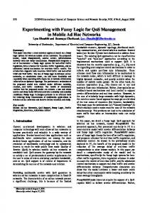
Figure 8 shows that labels 3, 8, and 5 were the hardest to classify correctly. Three of the top five classification pairs included the digit 3. This is intiuitive, due to the fact that it is similar in shape with 8 and 5. The easiest digit to classify appears to be 1. For these reasons we choose to classify 0-3 for the multiclass SVM, which includes the easiest and the hardest digits to classify. Unless specified otherwise, we only considered labels 0-3. This also allowed us to experiment with multiclass SVMs without being overburdened by computational complexity. The error rate when only considering two labels ranges from almost 0 to 9%. 5.3.2

Probabilistic SVM

The out-of-sample logistic classifiers consistently performed better then the other two. (See table 8) Furthermore, as the labeled set for the original SVM increased, the logistic multiclass classifier that was trained on that set became increasingly biased and over-fitted, which confirmed the results from [1]. This however, brings up an interesting point. We attempted to use this method for multiclass S3 VMs, and the assumption of S3 VMs is that the labeled set is rather small. The gain from increasing the labeled set for the original SVM compared to the gain from using the sigmoid function to classify the data is much greater. Unfortunately it does not make sense to use this method in a semi-supervised setting due to the scarcity of data. Our original hope was that the biased would not be large enough to affect the data as was hypothosised by Platt [1]. This however turned out not to be true. This shows a need for alternate methods for deducing the posterior class probability of a semi-supervised SVM. 5.3.3

Introduction of Unlabeled Data

An important aspect of our project is the effect of varying degrees of unlabeled data on a labeled set of a constant size. Our results are neither monotonically increasing or decreasing, but they do show a trend toward lower error with unlabeled sets of higher size. To see dramatic improvements though, it generally takes a large ratio of unlabeled to labeled data. Additionally, a larger labeled set improves results. As shown in figure 8, there is a dropoff in error rate at 120 unlabeled points versus 20 labeled points. This shows that in order to gain signifigant benefits from the unlabeled data, we need very large unlabeled data sets. However, due to the fact that increasing the size of the unlabeled set is very computationally 6

expensive, we were not able to run many experiments that used more than 200 unlabeled data points.

6

Conclusion

Although fitting a logistic function to generate the posterior probability for a given SVM greatly increases the accuracy of the classifier, we have found that in order to obtain good results, one requires a large out-of-sample labeled set to train the sigmoid function. This is due to the fact that training the sigmoid on the original labeled data set introduces a large bias. It is often better to use that data to train the original SVM function itself rather than using it to fit the sigmoid function. Futhermore, holding out a large amount of labeled data undermines the purpose of semi-supervised learning, which is often used in scenarios where that labeled data is scarse. We also found that our S3 VM implementation makes using unlabeled data quite computationally expensive. We weren’t able to perform many tests on a large unlabeled dataset, but our results do show a trend towards increased accuracy for larger working sets.

7 7.1

Individual Contributions Alex Gonopolskiy

For this project I helped write the paper, I wrote various matlab functions for multiclass, pca, working with the original data and converting it into various formats for easy use. I ran a number of experiments as well as helping my group members debug the code for thier parts.

7.2

Ben Nash

I wrote the S3VM model using the AMPL modeling language. I wrote the classify function in MATLAB which does the following: reads test parameters; creates datasets of the correct size using appropriate labels; for each classifier, writes data out in AMPL format, calls AMPL using appropriate commands, reads result into variables, classifies data; finds the highest classification; outputs the test error. Long and heavy editing and proofreading of paper.

7.3

Bob Avery

For this project, besides minor tings such as readin papers, assisting in debugging code, etc., I programmed a group of functions that read w, b and the test points from a file, classified them, and found the rate error rate for the test data. I also generated some of the data used in our report, with particular interest and effort in the differing error in pairwise differentiation. 7

7.4

Jeremy Thomas

One thing I did for this project was research various methods for classifying data points in multi-class situations, such as the probabilistic methods. Also, I helped run some experiments to generate some of the data used in our report.

References [1] J. Platt, “Probabilistic outputs for support vector machines and comparison to regularized likelihood methods,” 2000, pp. 61–74. [Online]. Available: citeseer.ist.psu.edu/platt99probabilistic.html [2] K. Bennett and A. Demiriz, “Semi-supervised support vector machines,” 1998. [Online]. Available: citeseer.ist.psu.edu/bennett98semisupervised.html [3] C. Hsu and C. Lin, “A comparison of methods for multi-class support vector machines,” 2001. [Online]. Available: citeseer.ist.psu.edu/hsu01comparison.html [4] X. Zhu, “Semi-supervised learning literature survey,” 2007, university of Wisconis - Madison. [5] O. Chapelle, M. Chi, and A. Zien, “A continuation method for semi-supervised svms,” in ICML ’06: Proceedings of the 23rd international conference on Machine learning. New York, NY, USA: ACM, 2006, pp. 185–192. [6] R. Fourer, D. Gay, and B. Kernighan, AMPL A Modeling Language for Mathematical Programming. Boyd and Frazer, Danvers, Massachusetts, 1993.

8

Appendix

8

Unlabeled Size 0 20 40 60 80 100 120 140 160 180

One Vs All .25 .24 .25 .26 .24 .27 .32 .18 .1965 .2310

Sigmoid Out .17 .2117 .25 .206 .254 .185 .24 .227 .1638 .17

Sigmoid In .28 .2968 .29 .29 .34 .34 .37 .2132 .2559 .24

Figure 1: Average error rates for labeled training size = 20

Effects of Unlabeled Data on Missclassification Rate 0.5 One vs All Sigmoid − Out of Sample Sigmoid − In Sample 0.45

0.4

0.35

0.3

0.25

0.2

0.15

0.1

0.05

0

0

20

40

60

80

100

120

140

160

Figure 2: Average Error rates for Labeled Training size = 20, the three plots compare the error rates for one-versus-all, sigmoid out-of-sample training and sigmoid in-sample training. The error rates gradually decrease as we add more unlabeled data points, and the sigmoid out of sample classifier consistently performs better than the other two.

9

180

Unlabeled Sigmoid Out 100 .1003 120 .0953 140 .0915 160 .089 180 .0828 200 .0752 Figure 3: Average error rates for labeled training size = 100. As the number of unlabeled points increases, the error rate slowly goes down. This points to the fact that to see a big contribution, one needs a large set of unlabeled points

Labeled Unlabled 0 20 120 0 40 120 0 60 120 0 80 120 0 100 120 0 120 120

Sigmoid Error 0.1722 .2412 0.1343 0.139 0.1273 0.1275 0.0988 0.0815 0.0932 0.1052 0.1125 0.109

Figure 4: Error rates for Semi-Supervised Vs Supervised. 120 unlabeled points were used and compared to zero or all of those points. As the number of classified points increased, the error rates for the semi-supervised learning tend to get lower then the fully supervised ones.

10

Figure 5: Error rates for five hardest and five easiest pairs of digits to classify. 3 appears a number of times as the hardest digit to classify and 1 appears as the easiest.

11