mission, large speed reductions with accompanying friction and backlash at joints ... the links, the backlash and friction present at the joint, and the nonlinearities ...
J. Indian Inst. Sci., Jam—Feb. 1996, 76, 109-124. Indian Institute of Science
Experiments and simulation of model-based controlled robots
ASHITAVA GHOSAL Department of Mechanical Engineering, Indian Institute of Science, Bangalore 560 012, India. Received on October 20, 1995. Abstract This paper presents an overview of a part of the work done in the Robotics and CAD Laboratory on the computational and experimental aspects of feedback control of mechanical manipulators. We first present experimental results which show that a feedforward, model-based controller performs significantly better than a proportional plus derivative (PD) controller. The experiments were performed at the Bhabha Atomic Research Centre (BARC), Bombay, on a complex five-degree-of-freedom manipulator, containing a four-bar mechanism for motion transmission, large speed reductions with accompanying friction and backlash at joints, and driven by AC servo motors. We next present simulation results which show that a simple two-degree-of-freedom manipulator undergoing repetitive motion, under model-based or PD control, can exhibit chaotic motions for a particular range of feedback gains and for large mismatch between the model and the actual parameters. Keywords: PD control, model-based control, uncertainties, chaotic motions, robots.
I. Introduction Most industrial manipulators are made up of links connected by rotary or sliding joint which allow relative motion between the links. One end of the robot is the fixed base and the other carries the end-effector or the tool. The robot joints are usually electrically driven by DC servo motors and they usually have sensors for feedback control and interaction with the environment. Most industrial manipulators and robots are controlled by the common proportional, derivative and integral (PID) control algorithm. It is, however, well known that a robot is a highly nonlinear system. The nonlinearities come from the change in inertia as a function of the configuration, coupling between the motion of the links, the backlash and friction present at the joint, and the nonlinearities due to flexibility at joints or transmission of motion from the actuators to the joint. Unlike in a linear system, there are no straightforward methods for choosing the gains of the controller for a robot and significant experimentation or tuning is required to obtain values of gains which results in acceptable performance of manipulators. Even after tuning it is observed that the accuracy and repeatability, damping and time response characteristics, steady-state error and other performance measures of a manipulator, under ND control, are not uniform throughout the workspace of the manipulator. To overcome this problem, researchers have proposed alternate control algorithms where the manipulator model (dynamic equations of motions) are used for 'feedback linearization'. In this arti-
•
ASHITAVA GHOSAL
110
cle, we discuss some experiments and simulations of model-based control of robots. The work presented here has been done by students at the Robotics and CAD Lab" and the experiments were conducted at the Bhabha Atomic Research Centre (BARC), Bombay. There exists significant literature on modelling of robots and experiments on modelbased control of robots 4-8 . There are two main differences between results reported in literature and the results reported in this paper. Firstly, the experiments were done on a complex five-degree-of-freedom robot, containing a four-bar mechanism to transfer motion to the third joint axis, and large speed reductions with accompanying backlash and friction at the joints. Secondly, unlike most robots mentioned in literature, the robot was driven by AC servo motors h 2 In this paper, we present experimental results for a 'feedforward' model-based controller, and compare the performance of model-based controller with the existing proportional plus derivative (PD) controller. It is clear from the experiments that the model-based controller gives better results than a PD controller. .
The robot under feedback (PD or model-based) control can be mathematically described by a set of nonlinear, coupled, ordinary differential equations. Many nonlinear equations are known to exhibit chaotic behaviour. Although there exists a vast body of literature on chaotic motions in Duffing's oscillator, inverted pendulum, maps and several other systems9s 10 , literature reports very few works on chaos in robots. A full review of literature is available in Srinivas 3 ; however, to the best of our knowledge, excepting Mahout et al." . 12 hardly any discussion exists robots on possible chaotic motions in feedback controlled robots. In this paper, we present simulation results of a simple, planar, two-degree-of-freedom robot, under feedback control (PD and model-based), undergoing repetitive motions. Although the robot is perhaps the simplest possible, it is still extremely difficult to derive any analytical results, and the only recourse is to perform extensive numerical simulations. From numerical simulations, we show that, for certain ranges of the controller gains and for large mismatch between the model and the actual robot parameters, the differential equations modelling the motion of the robot under feedback control can exhibit chaos. These simulations, apart from being of mathematical interest, can give lower bounds on controller gains for good performance of a robot. ,
The paper is organised as follows: in Section 2, we discuss briefly the modelling and feedback control of a robot. In Section 3, we describe some experimental results obtained from a PD controller and a model-based controller on a five-degree-of-freedom robot. In Sections 4 and 5, we describe some simulation results of a simple two-degree-of-freedom manipulator undergoing repetitive motions. Finally, in Section 6, we present the conclusions.
2. Mathematical model of a robot A serial robot is modelled as a sequence of rigid links connected by joints which allow relative motions between the links. One end of a robot is the fixed base and the other is free, carrying the end-effector or the tool. In a serial robot, the degrees of freedom at the joints determine the degree of freedom of the robot. For a general task involving arbitrary positioning and orienting the end-effector or the tool, a six-degree-of-freedom robot
EXPERIMENT'S AND SIMULATION OF MODEL-BASED CONTROLLED ROBOTS
roll
elbow
v.
ext ens i
:It
FIG.
11 1
Link
Length (m)
Mass (kg)
C.G. (m)
1 2 3 4 5
0.650 0.300 0.450 0.0 0.370
24.60 15.36 2.24 0.0 0.116
0.0 0.133 0.175 0.0 0.116
1. The schematic diagram of a 5-axis servo manipulator.
is required. The geometry and the kinematics of any serial robot is best described by the use of the well-known Denavit—Hartenberg parameters 4 . Usually, due to ease of actuation, only single-degree-of-freedom rotary or sliding joints are used, and most electrically driven robots are powered by DC or AC servo motors. Most robots also have sensors, such as optical encoders at the joints, to measure the joint rotation and for feedback control. Figure 1 shows a five-degree-of-freedom robot developed at BARC, and actuated by AC servo motors. The robot is equipped with optical encoders at the joints. 2.1. Dynamic equations of motion The dynamic equations of motion of an n-degree-of-freedom serial robot are a set of nonlinear, highly coupled ordinary differential equations. They can be obtained by several methods'', and can be written in a concise form as = [M(0)0 + C(0, +
g(0)± f(0,e)
(1)
where U (t) is the n x 1 vector of the joint variables, Pc, the n x 1 . vector of joint torques/forces, [M(6 )], the positive definite n x n mass matrix, C(6,64) . represent the Coriolis and centripetal terms, g(64 ) represents the gravity terms and f(O,e), the friction terms. 2.2. Trajectory planning The desired robot task can be planned in Cartesian space (in terms of a desired position and orientation of the end-effector) or in joint space (in terms of the desired motion at the joints). The desired trajectory for the joints, 0 d (t) can be obtained by using cubic polynomials and the joint angle, velocity and acceleration at a time t can be written as = a o + a t t + a2 t2 a3 t 3 Od (t) = a l + 2a 2 t + 3a3 t2 6
ed
= 2a2 + 603 t
ASHrTAVA GHOSAL
112
where ai , i = 1, 2,
, 4 are detcrmined using known initial and final states.
To enable a manipulator achieve a desired motion or task, we must choose a control algorithm which sends the torque commands to the joint actuators. The torques are usually computed continuously using feedback from the optical encoder at the joints. 2.3. PD and model-based control A common way to compute the joint torques is to use the well-known PD algorithm. The joint torques are computed as
d 6)+[1(](Od —
T = [K
(2)
where [K r] and [Kp ] are n x n diagonal, positive definite, derivative and proportional gain matrices. Often two additional terms are added on the right-hand side for improved performance and in such cases the control algorithm, known as a PID control algorithm, is given by T=
Od + [ k](t) d — 0) -F[K p ](0 d — 0) ÷{K f ol (I 9 d — 9)dt
(3)
The first term gives improved tracking performance and the last integral term can result in smaller steady-state errors. As mentioned earlier, a PD controller may not give uniform performance everywhere in the workspace of the robot. We next describe two such schemes in which the dynamic model of the robot is used to overcome this problem. 2.4. Computed torque and feedforward control algorithm According to the computed torque control algorithm 4, the joint torques are computed as
r
+
(4)
where we choose
[a] = m(e)] [
r' =9d -F[IC "in\
.7\
d 0)-1-[K
d—
where [M0],[g-,-)J, g•, and f(, ) are the estimated mass matrix, Coriolis and centripetal terms, gravity term and friction term, respectively. If the estimates and the actual model match exactly, it can be shown that the above control algorithm results in a set of linear, decoupled error equations, and in such a situation, the PD gains can be easily chosen (according to well-established linear control theory) to give uniform desired performance throughout the workspace of a manipulator. -
EXPERIMENTS AND SIMULATION OF MODEL-BASED CONTROLLED ROBOTS
113
In the case of a mismatch between the model estimates and actual parameters of the manipulator, the error equation is no longer linear and decoupled. However, the performance of the manipulator is expected to be better than with a PD control algorithm. To overcome the difficulty of computing the model in real time, one can precompute the model (using the known desired trajectory as opposed to the actual trajectory) and use it in a leedforward' manner. In this case, the control algorithm can be obtained using
.,..-----,
[aj=1,9 6 P = ge d ted)+,;( 9 )d+f(t 1d,td art = °d +[IC JO d — b) +frc je d —0).
(6)
In the next section, we present a comparison of implementation results for a PD and a model-based (feedforward) control scheme. Although similar implementation results for a direct drive arm with DC servo motors have been reported in literature's 8 the experimental results shown in this paper are for a more complex manipulator with a fourbar mechanism used for motion transmission from the actuators to the joint, large gear ratios with large backlash and friction at joints, and driven by AC motors. ,
3. Experimental setup and implementation results The robotic manipulator used in our experiments is shown in Fig. I. It has five revolute joints with a four-bar linkage used to drive axis 3. The table accompanying Fig. 1 gives the linkage dimensions, mass of the links and centre of gravity of each link. Unlike most of the electrically driven robots, this manipulator is actuated by two-phase AC motors. The AC motors are relatively heavy and they develop low driving torques at high speeds. Due to this, large speed reduction is required at each joint. Table I gives gear ratio and encoder ratio at different joints. The gears used for speed reduction are invariably accompanied by backlash and friction resulting in poor system response. A four-bar mechanism is used for transmission of torque from motor to the third joint. The motor which actuates the third joint is located remotely from the joint and toward the base of the manipulator. The four-bar mechanism considerably complicates the model of the structure but reduces overall inertia of the manipulator. Encoders are connected to the joints to measure rotation of the joint angle. Tachogenerators are attached to the motors to read the angular velocity of motors. Table I Transmission parameters Joint
Gear ratio
Encoder ratio
1 2 3 4 5
115.59 139.15 139.15 182.00 182.00
4 10 10 40/3 40/3
el'
ASHITAVA GHOSAL
114
35 30 25 V 20 15 t 4
lc
0
0.5
1
2
1.5
2.5
3
4
3.5
Time — seconds FIG. 2. Controller performance in following desired trajectory of joint.
•
We implemented two control schemes, the independent joint PD control and the feedforward, model-based control. The details of the model used in the model-based scheme are given in Gopal l and Ravikiran 2 . The actuator torques are given by T = T mdi
i-{K
d
+[1C
15)
where 'rpm( is the torque computed from the given trajectory and the dynamic equations of motion. The computed torques are converted to corresponding motor voltages with the
'-2 0 IL
tu 3 4 5 Time — seconds FIG.
3. Comparison of errors at joint 1.
EXPERIMENTS AND SIMULATION OF MODEL-BASED CONTROLLED ROBOTS
115
help of motor characteristics charts 2 . The model-based controller and PD controller were compared based on the performance of the robot. The experiments were conducted with different trajectories, sampling rates, time spans and friction compensation. We present one representative result. The manipulator is made to traverse from home position (0°, 0°, —90°, 180°, 0°) to goal position (30°, 40°,-60°,180°, 0 0 ) and back to home position in a span of 4 seconds and the joint values were computed at intervals of 5 ms (i.e., at a frequency of 200 Hz). Figure 2 shows the desired trajectory and the path followed by robot under model-based control and PD control. It can be seen from the figure that the trajectory followed using model-based controller is closer to the desired trajectory. Figure 3 shows error in 0 1 throughout the span of travel. The main error sources are backlash and friction; however, the error is small in the case of model-based controller due to dynamic friction compensation. The positional error was approximately —1°, in the case of a model-based controller but it was larger for the case of PD controller. For joint 2, the effect of gravity dominates over stiction and dynamic friction. Due to the absence of gravity compensation in the case of PD control, the arm fails to stay at home position (0 2 = 0) and falls rapidly below the desired position (Fig. 4). For joint 3 the performance was similar on both the controllers (Fig. 5). This is because the effect of the dynamics, -rind!, is smaller as one goes away from the base. It was observed that the manipulator, while operating under PD control, overshoots the goal position because of the absence of gravity and dynamic compensation. This resulted in the second joint impacting the mechanical stops. This was never observed when the manipulator was operating under model-based control. 3 2.5 gr.%
2
4 ;
1.5
g
1 i
I i
1 I 1.1. 1
1 i•••
•i
i
1
II /I 1b: ALS
„A
i
if
/
• • • • lic •
••
S eS
•• • • •• • • • •• • •
-it .
I 1 #.
•4
••••••1• • snli•••••t"
• • • • •ii,
i - 1.- 'PO --
•. :.,• : ,,
•
A
• . •.. •• • • •• • . •
i i I •••••••••••••••••••••4••••••••••••••••••.t
%
,
I• % 8 Vt g ; g • g .1 • act.
. :
I,
levy
$ tir •
st•It•
;
nit. • •• • • ••• so • • •••■ •• •• is. .. • • • •• • •• • w •• • • ie • • • a s i
1 !
• • •• • • •
411 • •
0.5
• • •• • • • ••
• • ••
i
•••• • •• • • • •• • ••• • • • .1. • • •
I .
.
1
1.5
...4 1.••••
2 Time — seconds
FIG. 4. Comparison of errors at joint 2.
••• • • •• 0 41 •••i• •••• • • •• • • •• • • • 9. • •
..•i_.•....•.... _4\
•• 1 t 3 I 1 It 3 1 1 1 3 •••••••106••••••••••••••••• • •••••••••••• 4.•••••••••••••••••••40 • ••••.....• •••
•••••
•
i 1 .!
••7 g 1 1. se 81 \IS i sari/lu g ........ Inell4p.g rigt • IF. •-
3
..1 -. .... ..i.....3.r........,. . / ..i ..,...,.............149dc 1.7.-.094
i . ••••.................1•••••......n.••
2.5
• ••••••••
3
3.5
4
ASH1TAVA GHOSAL
116
1.5 1 O. 5
g
P6 : I I I I OPeft I • i ° IS; •,04.4 : ! clrii i • •••!••••••••••••••••••••1••••••••••••••••••••1•••••••••••••••••••1•••••••••••••••••••••?•••••••••......... 9 • 1 I 1 sAti i' f kV ..000„ • 06 ..1 I i I 1 Itaik‘ I. i iI I iir• • ••••••••••• as • ••••40•• •••• ••••••••••••• 1 1 MOO now • no ••• NI •4411• • ••• Seas° • •• • VW • • • r ••• •••• •• •••• • • • • • • . .•••• •••• tr1111••• ••••• •••••••••••1 0. g 1 ■
■ •■ •■ •■
■
■
• 41
!tI
.. !I
vie( - based
PI.
g I mos. ....wan ...................4......•••• 00000 'Inv. 0....••••••• ■ •••••••It • ••••••••••• I I 8 I I B
i
I ri 4
i
•••••••••••••• • •• ••••••••••••• an • we •
4••■ •• •••
i
• ••••••••••••
$
•
-1.5 -2
I t i•
•
i t
i
I
I S
t I
t •• ••
i
met •••••••••)..••••• • . ,4
III i
.110 I
••••••
I
1!
I
.2
. . • . ...
SI
I a; jail l
I
• I • 1
!
1
7
• ••••••••• ■ ••••••• ■ ••
1140 . r
11161
: i ad : 10 • i
••••4•••••••••••••••••• •••••••••••••••••• ••••••••••••••••••••in•••••••••••••••••• ••••••••••••••••••••in•••••••••• ■ ••••••4•••••••••• ■■••••••••+ •••• 00000 0 a
•• • •t
0.5 FIG.
I
1I
ance••••••••••••••&••••••••••••••••••••4....5............1/...• . I t
1
1
.
••••• it ••••••••••••••••len•«••••••••••• • et•emas••••••
Is • i 1 •L S 1 i•
1
1i
II
00000
••••••••••••••••••040 ■ Onqtenags•S•••• ••••••••••••••••••••110••••••••• ■ ••11/44
••••••• ■ ••••• ■ •••
-1
.
a
I
I
1 3 3r
$ 1 a
t 1t
I
I S
7, I
_
1
5. Comparison of errors at joint 3.
1.5
2
2.5
3
3.5
Time - seconds
4. Possible chaotic motion in feedback-controlled manipulator As observed earlier, the equations describing the motion of a feedback-controlled robot are nonlinear. Several nonlinear equations are known to exhibit chaos for certain ranges of parameters. In this and the next section, we explore the possibility of chaos in a system of differential equations which model a feedback-controlled two-link robot with rotary (R) joints. The simple two-link robot, and not the five-degree-of-freedom manipulator, is chosen for simplicity in simulation and visualization of the results. Chaotic motions are a class of motions in deterministic physical and mathematical systems whose time history has sensitive dependence on initial conditions 9 . The sensitive dependence implies a divergence of slightly perturbed trajectories and hence long-term unpredictability. These types of motions occur in nonlinear differential equations for certain parameters, certain initial conditions and for repetitive motions. In this section, we consider a 2R planar robot under a PD and a model-based controller. We explore the possibility of chaos in the nonlinear differential equations describing the motion of this robot. The parameters of interest are the gains of the controller and the mismatch between the model and the actual robot. Although the system considered is very simple from a robotics point of view, it is still very difficult to do any analytical study on possible chaotic motions in this system. For this 2R planar robot, the corresponding dynamical system is of dimension te and is non-autonomous. It is very difficult to obtain any analytical results and only a numerical study appears to be feasible.
4
EXPERIMENTS AND STMULATION OF MODEL-BASED CONTROLLED ROBOTS
117
The dynamic equations of motion for a 2R robot can be written in the state space form as
= x2 = OM (X3 ))1K3 (X3 XK2 (X3 )4 + N2 (2X2X4, + 4))+N2 1)
K2(X 3 Yr 2
= x4 itt=
(
V3 (x 3
)) {—K 3 (xXK1 (xix x +x24 ))— K 2% (x 3, 1 + K 1%(x3) 2} 3/ 22 +K 2(Nx 3/( 2 x 24 (7) n
where the state variables are the joint variables e l , 02 and their derivatives, and
P3(X3)
=
de4M(x3
Ki (x3 ) = m1 r12 +1 1 +12 + m2r? + m 2q +2m 2 4r2 cos(x3 ) K2(X 3 ) =
m2d + 12 + m2 1i r2 cos(x3 )
K3 (X3) = m24r2 sin(x3 ) N2
= 12 + trt2d
(8)
In the above equations, mi , 1, , 1 and ri are the mass, length, inertia and location of the centre of gravity of link i, respectively. Figure 6 shows a sketch of the 2R robot under consideration. We consider two previously mentioned control laws, namely, (1) PD control and (ii) model-based control. The desired repetitive trajectories in the joint space are chosen as 0 =
A1 sin(to t)
(9)
0 d2 = A2 sin(co Physical parameters of the 2R robot Link Length Mass (kg) (m)
Yc XI
X0
FIG. 6. A schematic of a 2R planar rigid robot.
1 2
0.5 0.4
20.15 8.25
C.G. Intertia (kgn?) (m) 0.18 0.26
6.3 1.4
118
ASHITAVA GHOSAL
For the model-based control, we use eqns (4) and (5). Since the manipulator moves in a plane there is no gravity term and for simplicity we do not include the friction term. The gain matrices, [Kr ], [K,], are 2 x 2 constant, diagonal gain matrices. The estimates, [M(0)] and [C(0,9)], are computed by perturbing the robot parameters as follows:
=(l+ e)mi
where t > 0 implies an overestimated model and –1 0 1.85
•• •
3
U)
•
0' 2.5
3 3.5 Bifurcation Parameter KV
1.8 1.75' 3.65
4
EPS = —0.9 KP = 24
EPS = —0.85 KP = 18 0.4
5
IE
b
3.75 3.7 Bifurcation Parameter KV
0
>
—02
Co
Ct
(I) —5 2.5 FIG. I I
.
3 3.5 Bifurcation Parameter KV
4
3.65
3.75 3.7 Bifurcation Parameter KV
Bifurcation diagrams for the model-basec controller.
large (more than 0.6) and it was more easily seen for underestimations. For overestimations, it was observed only for very small values of Kp and K. This can be explained by realising that the 'effective' closed-loop gains are given by (Mr' fn if [Kp ] and [M1-1 fili[K,j. The 'effective' gains become large when e> 0 and are small when c < 0. Figure 11 shows the bifurcation diagrams of state variables x t and x3 for two sets of parameters. A bifurcation from period one to period two can be clearly seen. Again, it must be noted that the figures are a projection of the trajectory bifurcating in RA .
6. Conclusions In this paper, we have presented a brief overview of a part of the experimental and computer simulation work carried out in the area of model-based control of robots at the Robotics and CAD Lab at IISc, Bangalore. From the experimental work it is clearly shown that model-based control of a robot can greatly improve its performance. From the numerical study and results, we have demonstrated that the nonlinear, ordinary differential
EXPERIMENTS AND SIMULATION OF MODEL-BASED CONTROLLED ROBOTS
123
equations describing the motion of a feedback-controlled, rigid, planar, 2R robot undergoing repetitive motions can exhibit chaotic motions. We have shown that chaotic motions can occur for a range of gains and for large mismatch between model and the actual system. Although the range of controller gains, in particular the derivative gains, is far removed from usually critically damped (or overdamped) regime in any actual robot, this study, apart from being of mathematical interest, can give lower bounds on controller gains. The study can also help in obtaining conditions for better trajectory tracking in feedback-controlled robots.
Acknowledgments All the work described here has been done in the Robotics and CAD Laboratory by students. In particular, the experimental work was done by J. Ravikiran and T. K. V. Gopal. The simulation for exploring possible chaotic motions in feedback-controlled robots was done by L. Shrinivas. The experimental work would not have been possible without the hardware and help provided by scientists and engineers at BARC, Bombay. In particular, we acknowledge the cooperation and help provided by Dr T. A. Dwarakanath, K. Jayrajan, D. Venkatesh, Bhaumik, Mohan Das and M. S. Ramakumar.
References T. K. V.
Modelling and simulation of a 5-degree of freedom robot, M.E. Thesis, Deptt of Mechanical Engineering, Indian Institute of Science, Bangalore, India, 1995.
RAWKIRAN,
J.
Implementation of model based control scheme on a 5 degree of freedom robot, M.E. Thesis, Deptt of Mechanical Engineering, Indian Institute of Science, Bangalore, India, 1995.
3.
SHRINIVAS,
L.
Possible chaotic motions in a feedback controlled 2R robot, M.Sc.(Engng) Thesis, Deptt of Mechanical Engineering, Indian Institute of Science, Bangalore, India, 1995.
4.
CRAIG,
J. J.
5.
ASADA,
H.
1.
GOPAL,
2.
Introduction to robotics: mechanics and control, 1989, Addison— Wesley. AND SLOTLINE,
6. SpONG, M. W. 7.
AN,
C. Fl.,
J. J. E.
AND VIDYASAGAR, M.,
ATKE,s0N, C.
G.,
D. AND HOLLERBACH, J. M.
GRIFEiTHS, J.
8. KflostA, P. K. 9.
MOON,
F. C.
10. GUCKENHEIMER, 3. AND HOLMES, P.
Robot analysis and control, 1986, Wiley. Robot dynamics and control, 1989, Wiley. torque Experimental evaluation of feedforward and computed 1987, control, Proc. IEEE Conf. on Robotics and Automation, pp. 165-168. Real time implementation of computed torque scheme, IEEE Trans., 1989, RA-5,245-25 3 .
Chaotic vibrations, 1987. Wiley. Nonlinear oscillations, dynamical systems, and bifurcations of vector fields, 1983, springer-Verlag.
124
ASH1TAVA GHOSAL
1 1. MAHOUT, V., LOPEZ, P., CARCASSES, J. P. AND MIRA, C.
Complex responses(chaotic) of a two-revolute joints robot for periodical torque inputs, IFToMM-jc Int. Symp. on Theory of Machines and Mechanisms, Nagoya, Japan, 1992, pp. 221-225.
12. MAHOUT, V., LOPEZ, P., CARCASSES, J. P. AND MIRA, C.
Complex behaviours of a two-revolute joints robot: Harmonic, subharmonic, higher harmonic, fractional harmonic, chaotic responses, IFToMM-jc Int. Symp. on Theory of Machines and Mechanisms, Nagoya, Japan, 1992, pp. 201-205.
13. Kllost.A. P. K.
Real-time control and identification of direct-drive manipulators, Ph. D. Thesis, Deptt of Electrical and Computer Engng, Carnegie-Mellon University, USA, 1986.
14. GORDON, NI. K. AND SHAMPINE, L. F.
Computer solutions of ordinary differential equations: The initial value problem, 1975, W. H. Freeman.
15.
User's Manual IMSL MathILibrary, 1989.
16. WOLF, A., Swtn, J. B. SWINNEY, H. A. AND VASTANO, J. A.
Determining Lyapunov exponents from a time series, Physica D, 1985,16,285-317.
17. PARKER, T. S. AND CHU& L. 0.
Practical numerical algorithms for chaotic systems, 1989, SpringerVerlag.