Experiments on gravitational phase separation of binary immiscible

c 2007 Cambridge University Press J. Fluid Mech. (2007), vol. 591, pp. 289–319. doi:10.1017/S0022112007008257 Printed in the United Kingdom

289

Experiments on gravitational phase separation of binary immiscible fluids MISUZU SATO

AND

IKURO SUMITA

Division of Earth & Environmental Sciences, Graduate School of Natural Sciences and Technology, Kanazawa University, Kanazawa 920-1192, Japan

(Received 31 March 2006 and in revised form 7 July 2007)

We conduct experiments on gravitational phase separation of binary immiscible fluids using an oil–water mixture and study how the volumetric and viscosity ratios of the two phases control the separation process. First, we change the volumetric fraction of the two phases. We find that the initial phase separation rate depends strongly on the volumetric ratio of the two phases, and can be modelled by a buoyancydriven permeable flow using the Blake–Kozeny–Carman permeability formula. Next, we change the viscosity ratios of the two fluids, and we find that there are two distinct regimes with different styles of phase separation. Small viscosity ratio (100) cases are characterized by a diffuse lower boundary and a large vertical gradient of porosity. A polyhedral foam structure develops at the top of the mixture layer which is slow to rupture and to transform into a uniform oil layer. These differences can be interpreted to arise from a faster coalescence rate relative to the separation rate at high viscosity ratios. We simultaneously measured electrical resistivity in order to monitor the temporal change of the mean porosity in the mixture layer. The measurements were found to be consistent with the visual observation.

1. Introduction Gravitational phase separation of binary immiscible fluids is an important process during differentiation of self-gravitating planets. For example, the core formation process of the terrestrial planets occurs due to separation of iron from the magma ocean (Stevenson 1990). A magma ocean is a global-scale layer of molten rock which is likely to have formed during the early stages of planetary evolution by the heat generated from gravitational accretion (Safronov 1978). Several different modes of separation are possible: it can occur by rainfall of iron droplets from an iron–silicate mixture or from percolation of iron through molten or partially molten silicate. Important issues here are the time scale of core formation, the resulting vertical compositional structure of the mantle, the extent to which iron is retained in the mantle and the resulting core size. Another example is hydrogen–helium alloys at high pressures and temperatures. It has been suggested theoretically that helium droplets separate from an H–He mixture causing helium rainfall inside Jovian planets (Stevenson 1982). Gravitational energy released from the rainfall can become the source of the excess luminosity in Saturn and the presence of such layer can affect the magnetic field pattern (Stevenson 1980). Since iron alloys such as Fe–FeO, Fe– FeO–FeS are also known to have immiscible phase diagrams (Ohtani, Ringwood &

290

M. Sato and I. Sumita

Hibberson 1984; Urakawa, Kato & Kumazawa 1987), similar separation may occur in planetary cores and become an important energy source to drive the geodynamo. For these cases, the depth range at which the mixture layer forms has been constrained using a phase diagram alone, and it is important to know how the mechanical separation process modifies the structure within this depth range. In a smaller scale, magma such as basalts (Philpotts 1982) and carbonatites (Kjarsgaard & Hamilton 1989) are known to have binary immiscible phases as is evident from the microscopic textures. However there have been few attempts to interpret these textures in terms of fluid mechanics. Most previous works on phase separation of immiscible fluids have focused on this process in the absence of gravity (for a recent review, see Bray 2003). One of the few experimental works on gravitational separation processes is by To & Chan (1992, 1994) who used an isobutyric acid–water mixture as well as a 2-6-lutidine– water mixture and studied how the volumetric ratio affects the separation rate. Examples of other works are those by Cau & Lacelle (1993) who used an aniline– cyclohexane mixture and by Colombani & Bert (2004) who used an isobutyric acid–water mixture. For all these cases, the two immiscible fluids are formed by maintaining the temperature below the upper critical point of a phase diagram. In these experiments, the two phases were of comparable viscosity while planetary situations can have large viscosity contrasts. For example, an iron and silicate melt pair can differ by at least 2 orders of magnitude. In order to apply the phase separation to planetary situations, we need to extend the experiments to a regime of larger viscosity contrasts. Previous experiments have shown that gravitational phase separation of binary immiscible fluids is complicated, and to our knowledge, there is no complete theory or numerical calculations which fully simulates the phenomena that occur. In order to clarify the elementary processes operating in these experiments, it is instructive to compare them to simpler cases that are better studied. The problem of sedimentation of rigid particles has long been studied (see Davis & Acrivos 1985 for a review) but the detailed physics involved are still under current research (e.g. Segré et al. 2001). When many particles exist, fluid dynamic interaction between the particles increases the drag and the settling velocity becomes slower. Such hindered settling velocity has been measured as a function of the volumetric fraction of the particles and has been interpreted using numerical simulations (see Brady & Bossis 1988 for a review). Interaction between particles is also responsible for forming a sharp settling front, which has been observed in the separation of binary immiscible fluids as well. However droplets, unlike particles, are deformable and two adjacent droplets coalesce and rupture to form a uniform layer. Deformability allows droplets to form a very high volumetric packing fraction (∼ 1), larger than is possible for rigid particles (∼ 0.6). Drainage of the interstitial fluid between the droplets and subsequent coalescence have been well-studied (see Chesters 1991 for a review). These studies have shown that the drainage velocity depends on the viscosity ratio of the two fluids, and also that the flattening of the droplet interface slows fluid drainage and inhibits subsequent droplet coalescence. There have been a few works considering the case with more than two droplets (Lowenberg 1998; Lowenberg & Hinch 1996) but they were limited to a volumetric fraction of up to 0.3. A combination of sedimentation and coalescence has been simulated by Wang & Davis (1995) but it was assumed that the suspensions were dilute and that fluid dynamic interactions between droplets negligible.

Gravitational phase separation of immiscible fluids

291

Motivated by the geological interest, there have been studies on how a porous twophase medium with a deformable matrix expels the interstitial fluid from buoyancydriven permeable flow and compaction of the matrix (e.g. McKenzie 1984; Scott & Stevenson 1984). These works have focused on low porosity conditions, corresponding to high volume fraction of droplets, where the matrix forms a connected network, which is applicable only to the later stages of the phase separation process. A more realistic situation where there is a transition from a disconnected to connected network of matrices, has not been studied in detail. Furthermore processes such as droplet coalescence and rupturing have been neglected, for simplicity. In this paper we describe the results of a parameter study of gravitational phase separation of binary immiscible fluids. Instead of using two immiscible fluids forming a phase diagram, we use an oil–water mixture in which is easier to control the volumetric and viscosity ratios. We first summarize the parameters and non-dimensional numbers relevant to our experiments. We next present the results from a series of experiments in which the volumetric ratio of the two phases is varied for a fixed viscosity ratio using a salad oil and water mixture. We then present the results from a series of experiments in which the viscosity ratio of the two fluids using a silicone oil and hydroxyethylcellulose solution mixture is varied for a fixed volumetric ratio of 0.5. Here, we change the droplet and continuous-phase viscosity independently. These results are interpreted using simple physical models, and we consider the possible implications for geophysical situations.

2. Parameters and non-dimensional numbers In this section, we summarize the parameters and non-dimensional numbers relevant to our experiments. We review the previous works in terms of these numbers and clarify the parameter space of our experiments. First, we consider the droplet radius a. In our experiments, most of the droplet radii are in the range of 10−4 < a < 10−3 m. Droplet radius is relevant to the separation dynamics in several ways. One is that it controls the separation rate since permeable flow velocity is proportional a 2 as we discuss in detail in § 5.1. Another is that it controls the importance of Brownian diffusion, which can be measured using the particle Péclet number, V (2.1) Pe = D/a which compares the droplet velocity V to the Brownian diffusion velocity. Here, D is the diffusion coefficient (Landau & Lifshitz 1987) D=

kT , 6πηc a

(2.2)

where k is the Boltzmann constant, T is the absolute temperature and ηc is the dynamic viscosity of the continuous phase. In the present case, Pe ∝ a 4 . In our experiments and those of To & Chan (1992, 1994), Pe ∼ 106 . On the other hand, Péclet numbers were of the order of 1 and 10–100, in Cau & Lacelle (1993) and in Colombani & Bert (2004) respectively, because of the smaller droplet size (a ∼ 10−6 m). Thus our experiments can be considered to be in the regime where Brownian motions have negligible effect. Droplet size is also relevant to the magnitude of the interfacial surface tension. The importance of interfacial surface tension, which acts to restore the droplets to a

292


spherical shape, can be measured using the Bond number B=

ρga 2 γ

(2.3)

which compares the buoyancy to interfacial surface tension. Here ρ is the density difference between the two fluids, g is the gravitational acceleration and γ is the interfacial surface tension coefficient between the two fluids. In our experiments, B is of the order of 10−4 to 10−2 so droplets can be regarded as approximately spherical when they are not in contact with each other. However as already described, droplets deform when they approach each other and previous theoretical and experimental works on two interacting droplets have shown that such deformation starts to inhibit coalescence for a Bond number as small as B ∼ 10−3 for a viscosity ratio of 1 (Rother, Zinchenko & Davis 1997). Thus droplet deformation is also expected to become important in our experiments, and we intend to address how this becomes apparent when there are many interacting droplets. In our experiments, the volumetric fraction of oil ψ0 , and the viscosity ratio λ are varied. When oil droplets form, porosity is defined as φ0 = 1 − ψ0 . Similar to the case of sedimenting rigid particles, we expect the fluid dynamic interaction between the droplets to become important as the volumetric fraction of droplets increases, and to hinder separation rate, as has been confirmed in To & Chan (1992, 1994). The viscosity ratio λ is defined by ηd (2.4) λ= ηc where ηd and ηc are the dynamic viscosities of the droplet and continuous phases, respectively. In the limit of infinite viscosity ratio (rigid spheres), the spheres do not deform and droplet viscosity is irrelevant to separation dynamics. However, for finite viscosity ratio, droplet viscosity becomes important, because the drainage velocity of fluid between the droplets becomes a function of the viscosity ratio which in turn affects the coalescence efficiency (Chesters 1991). When the droplet deformation is neglected (i.e. droplets are always spherical), the drainage velocity of the film between the droplets decreases as λ increases due to the change in the boundary condition of the drainage flow (Davis, Schonberg & Rallison 1989). For low viscosity ratio (λ 1), the interface between the droplet and the continuous-phase fluid becomes stress free (fully mobile) and the drainage is fast due to plug flow. On the other hand, for high viscosity ratio (λ 1), the interface becomes rigid (immobile) and the drainage becomes slow due to parabolic flow. For intermediate viscosity ratios, the interface becomes partially mobile and the flow between the drops has contributions from both flows and the film drainage velocity decreases with λ as the contribution from parabolic flow increases and plug flow decreases. Such viscosity-ratio dependence of film drainage velocity has been confirmed from numerical calculations and experiments (Wang, Zinchenko & Davis 1994; Yoon et al. 2005). When the deformation of the droplets is considered however, the film drainage rate becomes very slow owing to flattening and dimple formation of the interfaces (Yiantsios & Davis 1990; Rother et al. 1997; Bazhlekov, Chesters & van de Vosse 2000). The deformation becomes significant as the interfacial surface tension decreases, and these calculations show that there is a critical capillary number, or equivalently a critical Bond number in the case of the present experiments, above which the coalescence is inhibited (Rother et al. 1997). In terms of parameter space, these studies have been done in the regime of small Bond numbers (10−4 < B < 10−1 ) and moderate viscosity ratios (10−3 < λ < 10) where


293

η (salad oil/water) ρ γ 58/1

84 23

Table 1. Properties of salad oil–water mixture used for the experiments with variable volumetric ratios. η (mPa s): viscosity, ρ (kg m−3 ): density difference, γ (mN m−1 ): interfacial surface tension coefficient.

small but finite deformation affects the film drainage and subsequent coalescence, assuming that the lubrication regime is established in the film. Recent studies have also explored larger Bond number (1 < B < 10) regimes (Kushner IV, Rother & Davis 2001) where droplet deformation becomes significant. However studies are lacking on the transition to very high viscosity ratio regimes (λ > 10) where droplets remains nearly rigid even upon approach but still deform when they touch each other, and also cases where there is a large population of droplets. Since the droplet interaction time is proportional to ηc and the droplet deformation time is proportional to ηd , the magnitude of droplet deformation decreases with viscosity ratio λ, because there would be insufficient time for the droplets to deform. In the limit of very large viscosity ratios, droplet deformation should become negligibly small (Lowenberg & Hinch 1997). To summarize, the viscosity ratio affects the boundary condition of the drainage flow as well as the degree of deformation. The combined effects of these two factors is unknown and we intend to study this from the experiments. Finally, in relation to our work, we briefly review the work by Wang & Davis (1995) who simulated the sedimentation of droplets by considering both gravitational and Brownian effects. They introduced a simple non-dimensional number Nr which compares the characteristic time scale of droplet sedimentation to that of collision, and defined it 3(1 − φ0 )H (2.5) Nr = 4a where H is the total height of the separating layer. In our experiments φ0 = 0.5, H = 0.14 m, a = 10−4 m from which we obtain Nr = 525. A value larger than unity indicates that there is sufficient time for the droplets to collide during separation. 3. Experimental method Two series of experiments are performed with different pairs of immiscible fluids. For the experiments with variable volumetric fraction, we use a salad oil (Nisshin Co., Japan) and distilled water coloured using a 0.01 wt% green fluorescent dye. The fluid properties for these experiments are summarized in table 1. For the experiments with variable viscosity ratios, we use a silicone fluid (Shinetsu Silicone KF96, Japan) with viscosity ranging from 0.82 to 12163 mPa s and a hydroxyethylcellulose (HEC) solution with a viscosity ranging from 1.0 to 185 mPa s. Here ion-exchanged water was used for the solution. Viscosity was measured using a rheometer (Brookfield DV2+ PRO). For a strain rate of the same order of magnitude as the separation rate, i.e. < 0.5 s−1 , HEC solution is a Newtonian fluid. Here, strain rate was estimated using the flow velocity in the interstitial channels between the droplets as the velocity scale and using the width of the channel as the length scale, which were obtained by assuming a permeability formula in equation (5.2) below and the permeable flow

294


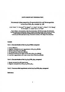
Figure 1. Experimental setup. In the experimental series with variable volumetric ratios, resistivity measurements are not performed and the volumetric ratio of the two fluids varies.

model (equation (5.5)). Silicone fluid was coloured using a 0.01 wt% yellow dye (Orient Chemicals Yellow 129). The HEC solution was coloured using a 0.0014 wt% blue food dye. These dyes only mix with their respective fluids, which enables us to monitor the phase separation process from the colour of the fluid. We also add 0.1 wt% NaCl to the HEC as an electrolyte and measure the resistivity of the fluid mixture to monitor the phase separation process. A summary of the experimental conditions for variable viscosity ratios is given in table 2. The interfacial surface tension between a pair of fluids was measured using a pendant drop technique. For the volumetric ratio dependence, the ratio of the two phases was varied in the range of 0.25 to 0.95. For the viscosity ratio dependence, the droplet (oil) to continuous phase (HEC solution) viscosity ratio was varied in the range of 0.0049 to 606. The interfacial surface tension between a pair of fluids with dye colouring and NaCl was the same as that without these additives, indicating that they do not act as surfactants. For each experimental run, we used a new set of two fluids because we found that the reproducibility of the experiments become poorer if we used the same set, possibly because after the experiment a fluid still contains minute droplets of the other phase. We also measured the interfacial surface tension for a pair of fluids corresponding to that of RUN66 of table 2, before and after the experiment, and found it to be the same within the accuracy of measurement. This indicates that any surface-active contamination of the fluids during the experiment is negligible. The experimental setup is shown in figure 1. We use a rectangular acrylic tank with an inner cross-section of 5 cm × 10 cm and a height of 18 cm. The experiments were done at room temperature. Resistivity measurements are made using an LCR meter (Agilent 4263B) at frequencies of 1, 10 and 100 kHz sampled at a period of 3 s. The electrodes are made of a stainless steel plate with a width of 3 cm and a height of 1 cm and are attached to the inner wall of the acrylic tank to measure the electrical impedance across the shorter cross-section of the tank (i.e. 5 cm). The experimental procedure is as follows. For the experiments with variable volumetric ratios, we fill the tank with specified volumes of oil and water to a total

295

Gravitational phase separation of immiscible fluids RUN 30 31 32 33 34 35 36 37 38 39 40 41 42 43 44 45 46 47 48 49 50 51 52 53 54 55 56 57 58 59 60 61 62 63 64 65 66 67

ηd

ηc

12163 12163 9710 9710 9710 9710 9710 5826 5826 5826 4855 4855 2913 2913 2913 2133 2017 2017 2133 971 971 971 971 485.5 485.5 485.5 485.5 485.0 339.5 339.5 96.6 48.1 48.1 48.1 28.7 9.4 0.82 0.82

23 22 21 23 35 86 170 22 101 163 24 102 22 105 185 4 20 19 109 3 22 21 22 1 3 24 22 65 3 21 21 1 1 20 23 24 20 168

λ 536 547 465 420 277 113 57.3 271 57.5 35.7 205 47.4 135 27.9 15.7 606 98.7 105 20 310 44.1 46.6 44.0 486 162 20.3 22.2 7.5 100 16.5 4.6 48.1 48.1 2.41 1.27 0.39 0.04 0.0049

ρ

γ

B

foam

LB

regime

31 31 34 32 35 37 37 33 35 37 33 35 33 35 37 31 33 33 35 31 32 33 33 31 31 33 33 39 32 33 38 41 41 43 49 69 186 190

40 35 34 34 21 22 24 23 24 21 22 23 21 21 17 36 18 17 19 20 20 16 13 29 13 17 13 14 14 14 12 17 17 19 17 11 7 6

0.0042 0.0043 0.012 0.0020 0.0027 0.0015 0.00083 0.0032 0.0014 0.00080 0.0019 0.0015 0.0019 0.00088 0.00047 0.0011 0.0049 0.0012 0.00052 0.0014 0.00055 0.0020 0.00092 0.027 0.0014 0.00048 0.0015 0.0025 0.0018 0.00085 0.00084 0.027 0.0089 0.00097 0.0014 0.0025 0.0073 0.0055

× × × × × × × × × × × × × × × × × × × × ×

D D D D D D D D D S D D D S S D D D S S S S S D S S S S S S S D D S S S S S

II II II II II II i II i I II i II I I II II i I i I I I II i I I I i I I II II I I I I I

Table 2. Summary of experiments with variable viscosity ratios. Here ηd (mPa s): droplet (silicone oil) viscosity, ηc (mPa s): continuous-phase (HEC) viscosity, λ: viscosity ratio, ρ (kg m−3 ): density difference, γ (mN m−1 ): interfacial surface tension coefficient, B: Bond number. The data are given in the order of decreasing droplet viscosity. Droplet size used for calculating Bond number is estimated using the data of the ascent of the lower boundary and the permeable flow model (equation (5.6)). Two criteria used to define the regimes are: (1) foam: indicate whether the foam structure is present near the upper boundary (denoted ). (2) LB: indicate whether the lower boundary is diffuse (D) or sharp (S). The three regimes are I, II and i (intermediate).

height of 14.2 cm. For the experiments with variable viscosity ratios and electrical impedance monitoring, we first fill the tank with HEC solution to a height of 14.2 cm and measure the electrical impedance of the HEC solution. We then replace half of the HEC solution with a silicone oil, so that the volumetric fraction of the silicone oil becomes 0.5. For both types of experiments, a high speed stirrer (Ika Eurostar Control

296


Visc) with a honeycomb structured stirring head designed to minimize incorporation of air bubbles (Ramond stirrer diameter 2.1 cm, Shiraimatsu Co., Japan), is used for mixing the fluid to form a uniform mixture. For the experiments with variable volumetric ratios, the rotation rate is fixed at 2000 r.p.m. For these experiments we confirmed that the droplet radius is unaffected by the volumetric ratio of the two phases. For the experiments with variable viscosity ratio, the rotation rate is changed from between 933 to 1999 r.p.m. to control the droplet radius, which is a function of shear rate and viscosity ratio (Larson 1999). We first start mixing the fluid at a low rotation rate to form a large uniform droplet radius and then gradually increase the rotation rate to form a smaller droplet radius. From measuring the droplet radius from microscopic images, we find that the average droplet radius is of the order of ∼10−4 m, with a polydispersity in terms of standard deviation of about 50% of the average radius. The statistics of the size distribution is characterized by a positive skewness. These properties were found to be common irrespective of rotation rate and viscosity ratio. After mixing, the tank is placed on a levelled plane (t = 0), and time-lapsed photos of the phase separation process recorded using a digital camera, which is then made into a movie. For microscopic observations at the droplet scale, we use a CCD microscope and a video recording system. These images were then analysed on a PC. 4. Results 4.1. Volumetric ratio dependence In this section we describe the results from a series of experiments with variable volumetric ratio of the two phases. For these experiments, we use a salad oil–water mixture and define the volume fraction of oil by ψ0 . In figure 2 we show examples of experiments for two different volumetric ratios: in figure 2(a) oil droplets are dispersed in water (ψ0 = 0.5) and in figure 2(b) water droplets are dispersed in oil (ψ0 = 0.7). We can identify oil and water droplets from their colour (oil is yellow and water is green) and from the topography of the boundaries. The presence of either type of droplets is confirmed from microscopic observations. From the experiments, we find that oil droplets form when ψ0 6 0.6 and water droplets form when ψ0 > 0.6. From the photographs, we can identify three layers during separation, which correspond to, from bottom upwards, a water layer, a mixture layer composed of oil and water, and an oil layer. We define the boundary between the oil layer and the mixture layer as the upper boundary (UB). In the case of oil droplets, the upper boundary is bumpy, owing to the small density difference and we use the largest height. In the case of water droplets, the upper boundary is a flat settling front owing to the large density difference. We define the boundary between the water layer and the mixture layer as the lower boundary (LB). In the case of oil droplets, the lower boundary is flat and well defined. On the other hand, in the case of water droplets, the lower boundary is bumpy and because of large droplet size it can vary laterally by as much as 1 cm. These factors cause a large uncertainty in defining the lower boundary. There is a well-defined flat boundary immediately above a layer of large water droplets and we define its height as LB . Since this height can be defined unambiguously, we use it to track the ascent of the lower boundary. The heights of these boundaries are indicated in figure 2 and are also shown schematically in figure 3. In the case of oil droplets, the lower boundary ascends due to ascending oil droplets and the upper boundary descends due to rupturing of oil droplets to form a uniform oil layer. On the other hand in the case of water droplets, upper boundary descends

297

Gravitational phase separation of immiscible fluids (a)

13 s

140 s

450 s

900 s

4055 s

(b)

25 s

1125 s

1710 s

2263 s

57802 s

Figure 2. Time-lapse photographs of the experiments with variable volumetric ratios using salad oil and water showing a section of the tank of height 14 cm and width 4.7 cm. The numbers indicate the elapsed time after the tank was placed on a levelled plane, immediately after the end of stirring. (a) Volumetric fraction of oil is ψ0 = 0.5, with droplets of salad oil dispersed in water. A three layered structure forms and the heights of the lower (LB) and upper boundaries (UB) are indicated by white and black circles, respectively and are used to plot figure 4(a). As time proceeds, the lower boundary ascends due to rising oil droplets and downward percolation of water. The upper boundary descends due to rupturing of oil droplets to form an oil layer at the top. The ascent velocity of the lower boundary is linear in time up to about t ∼ 600 s after which it slows down. (b) Volumetric fraction of oil is ψ0 = 0.7 and droplets of water are dispersed in oil. This is a grey scale image for the ease of visualization. The heights of the LB, LB and UB indicated by white open, white closed and black circles, respectively. Heights of LB and UB are used to plot figure 4(b). Upper boundary descends with time due to settling of water droplets and upward percolation of oil. Lower boundary ascends with time as the water droplets rupture to form a water layer at the bottom. Between LB and LB , the water droplets become large, of the order of 1 cm.

298


Figure 3. Schematic diagram illustrating the two cases of variable volumetric ratios using salad oil and water mixture. (a) Case where oil fraction is ψ0 6 0.6. Here oil droplets are dispersed in water. Oil droplets ascend and water percolates downwards. Heights of the LB and UB are used to monitor the separation rate and to calculate the mean porosity in the mixture layer. (b) Case where oil fraction is ψ0 > 0.6. Here water droplets are dispersed in oil. Water droplets sink and oil percolates upwards. Here LB is defined as the height of a flat interface immediately above a layer of large water droplets at the base of the mixture layer. Heights of the LB’ and UB are used to monitor the separation rate and to calculate the mean porosity in the mixture layer.

due to settling of water droplets and the lower boundary rises due to rupturing of water droplets to form a uniform water layer. These differences are also illustrated in figure 3. We track the heights of these boundaries from the photographs and plot them in figure 4. Using the heights of these two boundaries, we calculate the mean porosity (volumetric fraction of the continuous phase) φ in the mixture layer. In the case of oil droplets φ is calculated from φ(t) =

h0 − hLB (t) hUB (t) − hLB (t)

(4.1)

where hLB (t) and hUB (t) are the heights of the lower and upper boundaries, respectively, and h0 is the initial height defining the boundary between water and oil prior to stirring. In these experiments, the heights of the boundaries are measured to an accuracy of 0.25 mm which result in an error of 0.8–7% at the initial stage of separation and increases to 1.5 − 15% when the lower boundary has risen to half of the final separation height. The calculated error bars are shown in figure 4. Note also that the mean porosity in the mixture layer can either decrease or increase as the separation proceeds. If drainage at the lower boundary is faster than rupturing of oil droplets at the upper boundary, porosity decreases, and vice versa. From figures 2 and 4 we find that there are three stages during the total separation process. Here we describe these stages using figure 2(a) and figure 4(a).


299

(a)

Height (cm)

15 10 5 0

Mean porosity

0.5 0.4 0.3 0.2 0.1 0 101

102

103 Time (s)

(b)

Height (cm)

15 10 5 0

Mean porosity

1.0 0.9 0.8 0.7 0.6 0.5 102

103 Time (s)

104

Figure 4. Ascent and descent of the lower (LB) and upper boundaries (UB) and corresponding change of mean porosity in the mixture layer for the experiments in figure 2 using salad oil–water mixture. (a) Volume fraction of oil ψ0 = 0.5. Dashed and dash-dotted lines indicate heights calculated using constant and variable porosity model, respectively using (5.6). The droplet radius used for the model is the same for both cases (0.079 mm). (b) ψ0 = 0.7.

The first stage is the period immediately after stirring. At this stage, their is a vertically homogeneous oil–water mixture with no clear layered structure. In the case of oil droplets, from microscopic observation, we confirmed that oil droplets with a typical radius of the order of 10−4 m are ascending. The second stage is when the lower boundary appears and ascends at approximately a constant velocity. A well-defined boundary forms due to interaction between droplets. In figure 2(a), the lower boundary appears at t 10 s. On the other hand,

300


the upper boundary hardly descends at this stage, implying that drainage is faster than rupturing. As a consequence, the porosity decreases steadily. From microscopic observation of the mixture layer, we find that the permeable flow take the form of meandering channels whose lateral spacing is ∼10 droplet scales. As a result, some droplets were observed to be entrained downwards by the channel flow. Towards the upper boundary, droplet size become of the order of 1 mm, indicating droplet coalescence. The third stage is when the ascent velocity of the lower boundary slows down whereas the upper boundary starts to descend. In figure 2(a), this is the stage after t 600 s. Phase separation slows down and at t 4055 s, the mixture layer disappears and the separation is complete. For some experimental runs, the mixture layer was observed to collapse. The mean porosity in the mixture layer decreases steadily and approaches a minimum value of about 0.1, smaller than that of dense random packing (∼ 0.36) or hexagonal close packing (0.26) (Mavko, Mukerji & Dvorkin 1998). Such a low porosity is achieved from deformation of droplets and from smaller droplets filling the interstitial space of larger droplets. In the case of water droplets (figures 2b, 4b), water droplets coalesce efficiently before rupturing to form a uniform water layer. As a result, the droplets become large, of the order of 1 cm. Also the ascent and descent velocities of the lower and upper boundaries are similar and occur simultaneously. As a result, the mean porosity remains at a similar value throughout the separation process. From the measurements of the boundary heights shown for example in figure 4, we can calculate the ascent velocity. Since the ascent velocity is initially approximately constant, we use the data points up to one half of the final separation height and fit them by a line using a least-squares method, and use its slope to calculate the ascent velocity. Figure 5 shows the result as a function of the oil fraction. The ascent velocity decreases by approximately 2 orders of magnitude as the oil fraction increases from 0.25 to 0.95. Data shown for example in figure 4(a) indicate that the porosity in the mixture layer asymptotically approaches a minimum value which we define as the terminal porosity. Such a porosity can be interpreted to exist because the droplets resist further deformation by interfacial surface tension and thereby trap a finite amount of continuous-phase fluid. We can define the terminal porosity as the minimum porosity during separation and plot it in figure 6 as a function of oil fraction in the regime of oil droplets. In the case of water droplets, mean porosity does not decrease with time and a terminal porosity cannot be defined. The plot shows that the terminal porosity decreases with oil fraction ψ0 . Several qualitative reasons are possible for this. One is that the thickness of the mixture layer increases with oil fraction, which leads to a larger buoyancy and hence larger deformation of the droplets, which is preferred for decreasing porosity. Another is that the initial porosity decreases with oil fraction which implies that less continuous-phase fluid is expelled. 4.2. Viscosity ratio dependence In this section, we describe the results from a series of experiments with variable viscosity ratios using a silicone oil–HEC mixture. Here the volumes of oil and HEC are fixed and are identical (volumetric fraction 0.5). For all cases we find that the majority of the oil becomes the droplet phase and HEC becomes the continuous phase. We first describe the qualitative features of the separation and classify the regimes. We then describe a detailed analysis of the measurements of the boundary heights and resistivity.

301


Lower boundary ascent velocity (m s–1)

10–2

10–3

10–4

10–5

10–6 0

0.2

0.4 0.6 Oil fraction

0.8

1.0

Figure 5. Ascent velocity of the lower boundary up to one half of the total separation height as a function of volumetric ratios of oil ψ0 for experiments using salad oil and water mixture. Filled circles are for ψ0 6 0.6 where oil droplets are dispersed in water; open circles are for ψ0 > 0.6 where water droplets are dispersed in oil. Most of the error bars are smaller than the marker size. The solid line is the ascent velocity estimated from (5.5), using the measured droplet radius 0.1 mm and an empirical constant K = 15 in the Blake–Kozeny–Carman formula. 0.30

0.25

Terminal porosity

0.20

0.15

0.10

0.05

0

0.1

0.2

0.3 0.4 Oil fraction

0.5

0.6

0.7

Figure 6. Terminal porosity as a function of volumetric fraction of oil from experiments using salad oil and water mixture, for oil droplets (ψ0 6 0.6).

302

M. Sato and I. Sumita 0s

535 s

1018 s 1621 s 2950 s 4038 s 4883 s 8785 s

0s

(b)

0s

2345 s 3553 s 5485 s 12743 s 24576 s 38881 s 113509 s

0s

160 s

(c)

(a)

1853 s 3776 s 5583 s 8646 s 10071 s 11495 s 73227 s

400 s

520 s

882 s

1484 s 5417 s 11664 s

(d )

Figure 7. Time-lapse photographs from four phase separation experiments with different viscosity ratios using silicone oil–HEC mixture, showing a section of a whole tank. The vertical scale is 14.2 cm and the width is 2.6 cm. Volumetric droplet fraction is 0.5. The circles indicate the heights of the lower (LB) and upper boundaries (UB). In all of these cases, oil droplets are dispersed in HEC. The HEC layer at the bottom is blue, the mixture layer in the middle is green and the oil layer at the top is yellow. The numbers indicate the lapsed time after the tank was placed on a levelled plane, immediately after the end of stirring. The clear upper part of the oil layer in (b–d) is the settling front of water droplets which is a minor fraction. (a) λ = 0.4 (ηd = 9.4 mPa s, ηc = 24 mPa s), B = 2.5 × 10−3 (RUN 65). The lower boundary is sharp and a foam structure is absent. Note the approximately symmetrical ascent and descent of the lower and upper boundaries. Phase separation with these characteristics is classified into regime I. (b) λ = 20 (ηd = 486 mPa s, ηc = 24 mPa s), B = 4.8 × 10−4 (RUN 55: regime I). (c) λ = 58 (ηd = 5826 mPa s, ηc = 101 mPa s), B = 1.4 × 10−3 (RUN 38). The lower boundary is diffuse but there is no foam structure near the upper boundary. Phase separation with these characteristics is classified into intermediate regime. (d) λ = 271 (ηd = 5826 mPa s, ηc = 22 mPa s), B = 3.2 × 10−3 (RUN 37). The lower boundary is diffuse and there is a vertical gradient of colour in the mixture layer. The upper part of the mixture layer is yellow, and its thickness increase with time. This is a layer of low porosity with a polyhedral foam structure. Note also the asymmetrical ascent and descent of the lower and upper boundaries. Phase separation with these characteristics is classified into regime II.

4.2.1. Qualitative features of separation and the regimes In figure 7, we show the results of four phase separation experiments, in the order of increasing viscosity ratio. Similar to the experiments with salad oil and water, we can identify three layers during separation, which correspond to, from bottom upwards, a HEC layer, a mixture layer with oil droplets dispersed in HEC solution, and an oil layer. In the photographs, the layer of HEC is blue, the oil layer is yellow and the mixture layer as green. Similarly, we track the heights of the lower and upper boundaries and calculate the mean porosity in the mixture layer, which are plotted in figure 8. For these experiments, the boundary heights are measured to a maximum

303


Height (cm)

(a)

15 10 5 0

Mean porosity

0.5 0.4 0.3 0.2 0.1 0 101

102

103

104

Time (s)

Height (cm)

(b) 15 10 5 0

Mean porosity

0.5 0.4 0.3 0.2 0.1 0

102

103

104

105

Time (s)

Figure 8(a, b). For caption see next page.

accuracy of 5 × 10−6 m from digital images which results in an error of 0.02% at initial stage of separation and 0.04% when the lower boundary has risen to half the final separation height. In some cases, the lower boundary appears diffuse due to the vertically broad colour gradation. For these cases, we define the lower boundary as the height below which the colour of the fluid is uniform. The upper boundary is defined as the height above which oil droplets do not exist. Figure 8 shows that the lower boundary ascends smoothly, whereas the upper boundary descends irregularly due to the unsteady rupturing of the oil droplets. Figures 7(a), 7(b) are cases where the viscosity ratio is small (RUNS 65 and 55, respectively). Here the colour of the mixture layer is vertically uniform, which indicates that the vertical porosity profile in the mixture layer is approximately uniform. Also, the lower boundary remains sharp throughout the separation process as can be seen from figures 7(a), 7(b). From microscopic observation, we find that the droplet coalescence is slow and they remain of the order of 10−4 m radius. We also note

304


Height (cm)

(c)

15 10 5 0

Mean porosity

0.5 0.4 0.3 0.2 0.1 0 101

Height (cm)

(d)

102

103 Time (s)

104

105

102

103 Time (s)

104

105

15 10 5 0

Mean porosity

0.5 0.4 0.3 0.2 0.1

0 101

Figure 8. Height evolution of the lower and upper boundaries and the corresponding decrease of the mean porosity in the mixture layer for the four cases shown in figure 7. An irregular descent of the height of the upper boundary arises from the rupturing of oil droplets. Dashed and dash-dotted lines correspond to the height evolution calculated using constant and variable porosity models using (5.6) with the same droplet size. The droplet size is chosen to fit with the constant porosity model and is: (a) 0.202 mm, (b) 0.160 mm, (c) 0.314 mm, (d) 0.475 mm.

that the ascent and descent of the lower and upper boundaries occur simultaneously at a similar velocity, i.e. the two boundaries move symmetrically with respect to the final separation height. The photographs also show that a thin clear layer at the uppermost part of the oil layer emerges with time. This is a settling front of water droplets which constitute a minor fraction. We define the phase separation process with these characteristics as regime I. On the other hand, when the viscosity ratio is large (figure 7d) (RUN 37), there are significant differences. For this case, there is a vertical gradient of colour of the fluid in the mixture layer which indicates that the vertical gradient of porosity (i.e. the volumetric fraction of the continuous phase) is large. Also there is a vertical


305

gradient of droplet size, with larger droplets towards the upper boundary which take the form of a polyhedral foam. Furthermore, we observe that the lower boundary is initially sharp but becomes diffuse when the height of the lower boundary is about 5 mm from the bottom, and then later it becomes sharp again. In figure 7(d), we classify the images near the lower boundary from 160 s to 882 s as diffuse. Images from 1484 s to 5417 s show a transition from diffuse to sharp. These observations indicate that efficient droplet coalescence is occurring. When coalescence is efficient, larger oil droplets form and develop into a foam structure. Large droplets ascend quickly and small droplets are left behind, which causes a diffuse lower boundary. On the other hand, the descent of the upper boundary is slow and it remains at the same height during the period when the lower boundary ascends, i.e. the two boundaries move asymmetrically with respect to the final separation height. As a result, in the initial stages of separation, there are only two layers; the HEC layer and the mixture layer. Note also that the foam layer, which appears yellow in the photographs, becomes thicker with time as the HEC solution percolates downwards. In figure 9 (RUN 38) we show a close-up image of these structures at different heights. Figure 9(a) shows a large polyhedral foam structure near the upper boundary where the size of the droplets becomes as large as 1 cm. The structure closely resemble that of dry foams with a large volumetric fraction of air bubbles (Larson 1999). From the similarity we infer that the porosity (i.e. volume fraction of the continuous phase) near the upper boundary is < 0.05. Figure 9(b) is an image at the middle of the mixture layer indicating an upward coarsening of droplet size. Figure 9(c) is an image near the lower boundary, showing the vertical gradient of colour and the diffuse lower boundary. We define the phase separation process with these characteristics as regime II. A schematic diagram illustrating the differences of the two regimes is shown in figure 10. When the viscosity ratio is intermediate between the above two cases (figure 7c, RUN38), there is a regime which has the characteristics of both regimes I and II, i.e. where the lower boundary is sharp but a foam structure exists at the top or where the lower boundary is diffuse but a foam structure does not exist. In the example shown in figure 7(c), the lower boundary is diffuse but the foam structure is absent. For this example, images between 2345 s to 5485 s are classified as diffuse and after this the lower boundary becomes sharp. Note that the height at which the lower boundary becomes sharp is lower than that in figure 7(d). We define a phase separation process with these characteristics as the intermediate regime. We conducted a series of experiments by independently changing the droplet and continuous-phase viscosity. A summary of the experiments is given in table 2 together with the two criteria used to classify the experiments into regimes I, II or their intermediate form. Here, the diffusiveness of the lower boundary and the presence of a foam structure were identified from the movie made from photographs up to the time when the lower boundary height is 5 cm from the bottom. We classified the experiment as the case with a diffuse lower boundary (D), when there was a certain period during the separation process when the lower boundary became diffuse. For other cases, we classified the experiment as sharp (S). Another measure used for classification is the presence or absence of a polyhedral foam structure near the upper boundary with droplet size >5 mm. In order to minimize any arbitrariness of regime identification, both of the authors independently checked the images and agreed upon the classification. In figure 11 we plot the experiments given in table 2 in the parameter space of droplet viscosity versus viscosity ratio. The plot shows that the regime boundary is defined by the viscosity ratio, rather than the

306

M. Sato and I. Sumita (a)

(a)

(b)

(c)

(b)

(c)

Figure 9. Close up of a phase separation experiment in regime II λ = 536, ηd = 12163 mPa s, ηc = 23 mPa s, B = 4.2 × 10−3 (RUN 30) at approximately 210 s after the tank was placed on a levelled plane immediately after the end of stirring. The scale bar is 1 cm and corresponds to the length scale at the inner side of the acrylic tank. Left: A vertical section of a fluid layer with a height of 13.8 cm. Each box indicates the region where close-up images on the right were taken. (a) Polyhedral foam structure near the upper boundary. (b) Vertical structure in the middle of the mixture layer showing a vertical gradient of colour and droplet size. (c) Vertical structure near the diffuse lower boundary.

droplet viscosity. The viscosity ratio separating these two regimes is approximately 100. 4.2.2. Time evolution of the boundary heights and resistivity In this section, we describe how the lower and upper boundaries, mean porosity in the mixture layer and the resistivity change as the separation proceeds. Here, the resistivity is normalized to that of the continuous phase. Figures 12 and 13 are the measurements from regimes I (RUN 55) and II (RUN 37), and show how the heights of the lower and upper boundaries, the mean porosity in the mixture layer, and the corresponding resistivity changes with time. A plot is shown for the time interval during which the condition described in the Appendix, required to monitor the structure in the mixture layer, is satisfied. In the plot for the resistivity, we also draw a reference curve using Archie’s law and the mean porosity of the mixture layer. Archie’s law is an empirical relation between resistivity and porosity, and is given by σ = φ −m (4.2) σ0

307


Figure 10. A schematic diagram illustrating the characteristics of (a) regime I (λ < 100) and (b) regime II (λ > 100) for the experiments with variable viscosity ratios using silicone oil and HEC mixture. Arrows represent the direction of permeable flow. 105

Droplet viscosity (mPa s)

104

103

102

101

100

10–1 10–3

10–2

10–1

100

101

102

103

Viscosity ratio

Figure 11. Parameter space of the experiments with variable viscosity ratio λ, plotted as a function of droplet viscosity and viscosity ratio for all the experiments shown in table. 2. The diagonal array of points corresponds to the case where the viscosity of the continuous-phase fluid (HEC) is fixed at ηc = 22 ± 1 mPa s. Open squares: regime I; grey triangles: intermediate regime; solid circles: regime II. The plot shows that the regime boundary is defined by the viscosity ratio.

where σ is the resistivity of the mixture, σ0 is the resistivity of the continuous-phase fluid, m is an empirical constant and φ is the porosity (for a review, see Friedman 2005). Hanai (1968) theoretically derived m = 1.5 for electrically insulating spherical

308 Height (cm)

M. Sato and I. Sumita 15 10

(a)

5

Resistivity

Mean porosity

0 0.4

(b)

0.2 0 10

(c)

5 0

0

2000

4000

6000

8000

10000

Time (s)

Figure 12. An example of the time-series data for a case in regime I (RUN 55) for the time interval during which the condition described in the Appendix is satisfied, showing part of the data in figure 8(b). Here λ = 20.3 (ηd = 486 mPa s, ηc = 24 mPa s). (a) Time evolution of the heights of the lower and upper boundaries shown as solid line with points. Dashed and dash-dotted lines indicate the heights calculated using constant porosity and variable porosity model, respectively using (5.6). (b) Time evolution of the mean porosity in the mixture layer shown as a solid line with points, and that calculated from the variable porosity model as a dotted line. (c) Time evolution of the resistivity measured at 100 kHz shown as a bold line. Measurements at 1 and 10 kHz overlap the measurements at 100 kHz and are not plotted. The line with points indicates the model result using a mean porosity and Archie’s law with an exponent m = 1.5. The measured resistivity is slightly larger than that estimated from the model.

droplets in a conductive continuous phase, and we use this value to draw the reference curve For both figures 12 and 13, at t = 0, the measured resistivity agree well with that estimated using Archie’s law and the mean porosity. For figure 12 (regime I), the agreement is good throughout the period shown. On the other hand in figure 13 (regime II), as time proceeds, the measured resistivity becomes smaller than that estimated using Archie’s law and mean porosity. In figure 14 we plot the results from all experiments in the form of normalized resistivity (σ/σ0 ) versus mean porosity of the mixture layer with three different colours corresponding to the three regimes. Here we interpolated the time-series data of porosity to synchronize with the resistivity measurements. Since resistivity increases as the porosity decreases during separation, the trajectory of the data points moves towards the upper left corner of the plot with time as shown by an arrow. At φ = 0.5, although there is some scatter, the √ resistivity is similar to or larger than the value of 2 2 2.8 estimated using Archie’s law with an exponent of m = 1.5. One possible reason for a tendency for a larger value than 2.8 could be flattening of the droplet interface due to deformation. Resistivity values of fused glass beads, similar to the situation in our experiments give a larger value of m (Friedman 2005). As separation proceeds, we find that the trajectory follows a different path according to the regime. Cases in regime I are generally characterized by a steep slope and hence a relatively large resistivity as time proceeds. Cases in intermediate regimes are characterized by a slope which agrees

309

Height (cm)

Gravitational phase separation of immiscible fluids 15 (a)

10 5

Resistivity

Mean porosity

0 0.4 (b) 0.2 0 10

(c)

5 0

0

200

400

600

800

1000

1200

1400

1600

Time (s)

Figure 13. As figure 12 but for a case in regime II (RUN 37), showing part of the data in figure 8(d). Here λ = 271 (ηd = 5826 mPa s, ηc = 22 mPa s). In (c) the measured resistivity is smaller than that estimated from the model. 10 9 8 7

Resistivity

6 5

4

3

2 0.2

0.3

0.4

0.5

Mean porosity

Figure 14. Measured resistivity normalized by that of the continuous-phase resistivity, versus mean porosity in the mixture layer. Each line represents one experimental run using data shown for example in figures 12 and 13. Here mean porosity is calculated from the heights of the lower and upper boundaries using (4.1). As separation proceeds, the data points move towards the upper left corner as indicated by an arrow. Solid blue, broken black and solid red lines are experiments from regimes I, intermediate and II respectively. Black solid line indicates the Archie’s law dependence of resistivity as a function of porosity (4.2) using a power law exponent of m = 1.5. Here the data points are plotted for the time interval during which the condition given in Appendix is satisfied.

310

M. Sato and I. Sumita Height (cm) UB

LB

0

0.4 Porosity

1

Figure 15. A schematic diagram showing the difference in the vertical porosity profile for regimes I and II. Solid and dotted lines indicate vertical porosity profiles inferred from the photographs and resistivity measurements, for regimes I and II respectively. The height of the electrodes is shown on the left together with the height range indicating the effective region of the electrodes as broken lines. The photographs are the typical examples from regimes I (RUN 55, left) and II (RUN 37, right) both of which are at the time when the mean porosity in the mixture layer is 0.4.

well with that calculated using m = 1.5. Cases in regime II are characterized by a small slope and hence a relatively small resistivity as time proceeds. In figure 15, we show a schematic diagram of the vertical porosity profile of the two regimes inferred from the images and resistivity measurements. Here we compare two cases with the same mean porosity (0.4) in the mixture layer but for different viscosity ratios. In regime I, from the vertically uniform colour, we infer that porosity is nearly uniform in the mixture layer except near the top, which appears yellow in the image. On the other hand, in regime II, there is a thick foam layer at the top. Furthermore, from the vertical gradient of the colour in the mixture layer, and from a smaller resistivity, we infer that the porosity is large compared to regime I in the lower half of the mixture layer. As a consequence, on comparing the vertical profile for regimes I and II, a crossover of porosity is inferred to exist in the mixture layer. Also, the diffuse nature of the lower boundary suggest that there is a boundary layer of porosity near the lower boundary. These features are illustrated in figure 15.

5. Discussion 5.1. A model of the ascent velocity of the lower boundary We can model the ascent of the lower boundary using permeable flow in the frame of reference where droplets are stationary (To & Chan 1992; Faber 1995). Darcy’s law


311

relates the non-hydrostatic pressure gradient to the volumetric permeable flow rate per unit area, v, Kφ dP v=− (5.1) ηc dz where Kφ is the permeability and ηc is the continuous-phase viscosity, and z is taken positive upwards. For permeability, we use Blake–Kozeny–Carman equation (Dullien 1979) a2 φ3 . (5.2) Kφ = K (1 − φ)2 Here a is the droplet radius and K is a constant which depends on the tortuosity of the porous medium and φ is the porosity. In our experiments, droplets radius varies but it is known that (5.2) can still be applied if average particle radius a¯, defined as 1 fi , (5.3) = ai a¯ i is used, where fi is the volume fraction of the droplets with size ai (Mavko et al. 1998). The non-hydrostatic pressure gradient in the mixture layer near the lower boundary can be expressed as dP (5.4) = ρg(1 − φLB ) dz where ρ is the density difference between the droplet and the continuous phase, g is the gravitational acceleration and φLB is the porosity near the lower boundary. Here the pressure gradient is positive upwards because it balances the buoyancy of the lighter droplet (oil) phase. Since v is the volumetric flow rate per unit area, and the lower boundary ascends as the continuous phase percolates downwards, the ascent velocity of the lower boundary is from (5.1)–(5.4) VLB = −v =

KφLB (1 − φLB )ρg. ηc

(5.5)

Darcy’s law is known to be applicable when droplet Reynolds number = Va/ν < 10 (Bear 1972). In the experiments with salad oil and water, maximum droplet Reynolds number is estimated by taking V ∼ 10−3 m s−1 , a typical droplet radius a ∼ 0.1 mm and ν ∼ 10−6 m2 s−1 , as Re ∼ 0.1, thus validating using Darcy’s law. The droplet Reynolds numbers for experiments with HEC and silicone oil are smaller than this value because of the higher viscosity of HEC. Using a 10−4 m obtained from microscopic observations, we calculate VLB as a function of φ and draw the theoretical curve in figure 5. Here empirical constant K in (5.2) is an integer chosen to best fit the data points for the regime of oil droplets (ψ0 6 0.6) where permeable flow model is applicable. We fit the data using a nonlinear least-squares method and find that K = 15 ± 0.5 best fits the data. This value for K is of the same order of magnitude as the estimate by Bear (1972) who give a value of K = 45. The smaller value may be due to the localized channel flow observed microscopically which causes a larger effective droplet size or equivalently a smaller value of K. For the water droplet regime (ψ0 > 0.6) the model tends to underestimate the experiments. In this regime, the ascent of the lower boundary occurs due to rupturing of water droplets, and a permeable flow model is not appropriate to model this process. As an alternative we also tried the Rumpf–Gupte permeability formula (Dullien 1979) and found that it also gave a good fit to the results.

312


We can calculate the time evolution of the height of the lower boundary by specifying the porosity and permeability at the lower boundary and numerically time integrating the lower boundary velocity given by (5.5) and using (5.2): ρg a 2 t φLB (t)3 h(t) = dt. (5.6) ηc K 0 (1 − φLB (t)) We assume that the droplet size at the lower boundary is constant, which is confirmed to be a valid approximation from microscopic observations. For the constant in the Blake–Kozeny–Carman equation we use K = 15 obtained from figure 5. Here, two simple end-state cases can be considered for porosity φ at the lower boundary. One is where the porosity is fixed at the initial value φLB (t) = φ0 (constant porosity model). This can be considered to be a good approximation at the initial stages of separation and gives the upper limit estimate. The other is where the mean porosity between the lower boundary and the top of the fluid layer is used for the estimate of φLB (t) (variable porosity model). In the latter model, φLB (t) decreases as the lower boundary ascends. This becomes a better approximation as separation proceeds and the porosity at the lower boundary decreases, and can be considered to be a lower limit value, assuming that the porosity decreases monotonically with height in the mixture layer. The optimum estimate of the droplet radius is obtained from the model using a least-squares fit of the data points up to a height of 3.5 cm (i.e. half of the final thickness of the HEC layer). Note that this droplet radius would correspond to the effective droplet radius defined in (5.3). We tried both models and found that for most experiments, the constant porosity model gives a better fit because the lower boundary initially ascends linearly with time, and use this model to calculate the droplet radius. Examples of the fits are shown in figures 4, 8, 12, and 13. Here results for both constant and variable porosity models are plotted using the droplet radius chosen to fit the constant porosity model. From these figures, we find that the experimental measurements of the lower boundary heights are within the estimates from these two simple models. At later stages when the lower boundary ascent velocity becomes slower, the experiments agree better with variable porosity model. This is also evident from the reasonable agreement of porosity calculated from the heights of the boundaries and from the variable porosity model. The two end-state models described here are simple and do not model the height-dependent porosity structure, which becomes important as separation proceeds. However we consider that these two models serve as starting points for further detailed numerical models. 5.2. Regime diagram and its interpretation In this section we first summarize our experiments in the form of a regime diagram, and then consider the mechanism which gives rise to the different regimes. The two non-dimensional numbers characterizing our experiments are the Bond number, equation (2.3), and the viscosity ratio of the two phases λ (equation (2.4)). We can relate the Bond number to the capillary number, which compares the viscous stress to interfacial surface tension, as Kφ (1 − φ)B (5.7) Ca = a2 by using the velocity scale in (5.5). In order to calculate Bond number, we need an estimate of the droplet size and use the permeable flow model described in § 5.1 for the calculation. As shown already in figures 4, 8, 12 and 13, the constant porosity

313

Gravitational phase separation of immiscible fluids 103

102

Viscosity ratio

101

100

10–1

10–2

10–3 10–4

10–3

10–2

10–1

Bond number

Figure 16. Regime diagram for the silicone oil–HEC mixture experiments given in table 2. Open squares: regime I; grey triangles: intermediate regime; solid circles: regime II. A dotted line indicates λ = B −0.5 and is drawn as a reference (see text for details).

model gives a better fit to the experimental result than the variable porosity model at the initial stages, so we use the constant porosity model to calculate the initial droplet size. The estimated droplet size is confirmed to agree with the size obtained from microscopic observations. The calculated Bond numbers for each experiment are given in table 2. In figure 16 we plot the experimental results in the form of a regime diagram as a function of Bond number and viscosity ratio, indicating the two regimes and their intermediate one. We next consider the mechanism which give rise to the regimes. Our experiments suggest that the ratio of two velocity scales, the velocity of the coalescence of two adjacent droplets and the velocity of the gravitational phase separation, determines the two regimes. When this ratio is small, droplet coalescence is slow and results in regime I and vice versa for regime II. As described in § 2, droplet coalescence is controlled by drainage velocity which is proportional to f (λ)/ηc and is a function of viscosity ratio λ. On the other hand, we showed that the separation velocity can be approximately modelled using a permeable flow which is proportional to 1/ηc . There are two competing factors which determine f (λ). The first is the change in droplet interfacial boundary condition that causes the drainage velocity to decrease with λ. The second is the change of the degree of deformation which inhibits drainage and is a decreasing function of λ. When the effect of boundary condition alone is considered (i.e. deformation neglected), the film drainage velocity normalized with the permeable flow velocity depends on λ as shown by a broken line in figure 17. However, when the droplet deformation is considered, drainage is slowed at intermediate λ values, and based upon our experiments, we infer that the broken line in figure 17 would be qualitatively modified to the solid line. Note that we inferred that there is a λ range where droplet coalescence efficiency increases with λ. We interpret that, in our

314


Vd/Vp Fully mobile I

II

Immobile

λc Fully mobile

Partially mobile

Viscosity ratio Immobile

Figure 17. A diagram showing the viscosity ratio dependence of coalescence efficiency Vd /Vp at B < 1. Vd is the drainage velocity of the film between the droplets, and Vp is the permeable flow velocity during phase separation. The broken line indicates the case where droplet deformation is neglected. For this case, the droplet is always spherical and the coalescence efficiency decreases with viscosity ratio as the interface between the droplet and the continuous-phase boundary transforms from fully mobile to immobile as shown schematically at the bottom. The solid line indicates the case where droplet deformation is included. For this case, the droplet interface flattens and dimple forms, as shown schematically at the top and the film drainage is strongly inhibited. λc is the viscosity ratio above which a droplet can be considered to be nearly rigid and deformation can be neglected. Our experiments suggest λc ∼ 100 and that regimes I and II approximately correspond to the ranges shown by the arrows.

experiments, the critical viscosity ratio above which the droplet deformation becomes negligibly small is λc ∼ 100. We note that there is a transition of interfacial mobility from immobile to mobile as the droplets approach each other (Davis et al. 1989) because of the increase of the shear stress exerted at the boundary by the drainage flow. One criterion for an immobile interfacial boundary was obtained by Yiantsios & Davis (1990). They showed that for λ B −1/2 , the interface remains immobile even when the droplets approach so close to each other that the droplet deformation becomes significant. This criterion can also be restated as the condition where drainage occurs primarily under an immobile boundary condition, and we draw this line in figure 16 as a reference. Comparison shows that the regime boundary lies within an order of magnitude of this reference line, from which we infer that the inhibition of film drainage by droplet deformation is most significant in the intermediate viscosity range where the interface is partially mobile (figure 17). Future theoretical study is needed to verify this. There are several other factors that need consideration. One is the effect of surfactants which rigidify the interface regardless of viscosity ratio. In order to confirm that dye and NaCl does not act as surfactants, and that the resulting regimes are unaffected by these additives, we conducted separation experiments without dye


315

and NaCl. We confirmed that the features of regimes I and II are reproduced when the viscosity ratio is varied, even in the absence of these additives. A second factor is that the regime boundary shown in figure 16 may be shifted when a pair of fluids that are different from the silicone oil–HEC solution pair are used. In our experiments with variable volumetric ratios using salad oil–water mixture, the viscosity ratios for the cases of oil droplets and water droplets are λ = 58 and λ = 0.017, respectively. Experiments for λ = 58 show characteristics of regime I of silicone oil–HEC experiments, and are consistent. However, the results for λ = 0.017 show significant droplet coalescence and are quite different from the silicone oil–HEC experiments with comparable viscosity ratio. A regime of efficient droplet coalescence at low viscosity ratio is inferred as shown schematically in figure 17 and it is possible that the viscosity range below which this regime becomes apparent is larger for the salad oil–water pair than the silicone oil–HEC pair. We consider that the additional parameter that is different for the two sets of pairs is the effective Hamaker parameter Aeff which is a measure of the van der Waals force and is responsible for droplet coalescence: 1/2 2 Aeff = A1/2 , (5.8) oil − Aw where Aoil and Aw are Hamaker parameters of oil and water, respectively. It is known that the values of Aeff for the silicone oil–water pair is an order of magnitude smaller than that for the hydrocarbon-water pair (Koh et al. 2000). Thus the critical film thickness for droplet coalescence is larger for the salad oil–water pair, which explains the efficient droplet coalescence for this pair. 5.3. Comparison with previous works Experiments by To & Chan (1992, 1994) were done at a similar Bond number as in our experiments but at a viscosity ratio of the order of 1. Their results show that the upper and lower boundaries move simultaneously and linearly in time, consistent with the features of regime I in our experiments. In our experiments and in those by To & Chan (1992, 1994), the droplet radius near the lower boundary remained constant. This is in contrast to the experiments by Cau & Lacelle (1993) and Colombani & Bert (2004) which indicated a droplet growth. This difference possibly arises from the pronounced Brownian diffusion due to smaller droplet size in their experiments. Droplet coalescence in regime I of our experiments is slow, and the results can be compared with the phase separation of a deformable porous medium which assumes that the droplet size is constant and does not evolve with time (McKenzie 1984; Scott & Stevenson 1984). An example of a solution for an initially uniform porous medium undergoing deformation and expelling interstitial liquid is given in Spiegelman (1993). A solution obtained shows a smoothly decreasing porosity with height, similar to the situation of regime I in our experiments. 6. Geophysical implications Although our experimental parameter range is restricted compared to geophysical situations and simplified (e.g. no phase change, heat transfer or convection) some insights can be given. First, consider a magma ocean consisting of a mixture of immiscible silicate (> 0.1 Pa s) and iron melts (∼ 10−3 Pa s). Here we use the lower limit for the viscosity of silicate melt because it is strongly temperature dependent and increases with cooling. When iron droplets descend in a silicate melt, the viscosity ratio becomes λ 6 10−2 ,

316


whereas when iron melt percolates through ascending silicate droplets, λ > 100. In a convecting magma ocean, droplets are subject to shear, and as a consequence the Bond number should remain B 6 1 (Stevenson 1990), and the droplets eventually settle to form a mixture layer because convective velocities diminish near the bottom boundary layer (Martin & Nokes 1988). This corresponds to a droplet radius of a < 5 × 10−3 m for Earth where we use ρ ∼ 4500 kg m−3 (Stevenson 1990) and γ ∼ 1 N m−1 (Keene 1995). These values of B and λ are roughly in the range of those in our experiments. Now we consider the implications regarding the time scale, the style of core formation, the resulting core size and the degree of stratification of the mantle. Our experiments show that given the droplet size and viscosity of the continuous-phase fluid, the growth rate of the core can be approximately estimated using the permeable flow as has been done previously (Solomatov 2000). However, our experiments also show that complete separation is rate limited by the slow rupturing of droplets to form a uniform layer. If freezing occurs before separation is complete, some fraction of iron would be retained in the mantle. Our experiments show that the variation of iron content with height above the core–mantle boundary can be quite different depending on whether iron or silicate droplets form, and on the cooling rate of the planet. If the core formation occurs by iron melt percolation through silicate droplets, the mantle can become strongly stratified, and because the iron melt forms a network, an electrically and thermally conductive layer would form at the base of the mantle. Also, since freezing is faster for smaller planets, we may associate a structure like that at t = 160 s and t = 11664 s of figure 7(d) with the resulting structure in asteroids and terrestrial planets respectively. We also note that conventional theories of core formation have hardly considered the possibility of rising silicate droplets and downward percolation of iron melt, corresponding to large λ cases in our experiments. However, simple force balance arguments show that the critical volumetric fraction below which the more viscous phase becomes droplets is ∼ λ/(1 + λ) (Onuki 1994). If this is applicable to a convecting magma ocean, then the more viscous silicate phase would form droplets unless its volumetric fraction is close to 1, suggesting that this mode of separation can occur. Next we consider binary immiscible silicate melts, and consider how our experiments may be related to interpreting actual rock textures. The viscosity of silicate melts depends strongly on silicate content. In the case of basalts, the two immiscible phases are the Fe-rich (Si ∼ 40 wt%) phase and Si-rich (Si ∼ 70 wt%) phase. Using the results of Bottinga & Weill (1972), we can estimate the viscosity contrast for this pair of fluids to be of the order of 105 . In the case of carbonatite magmas, the two phases are carbonate-rich (Si ∼ 1 wt%) phase and silicate-rich (Si ∼ 30 − 40 wt%) phases, for which we similarly estimate a viscosity contrast of the order of 100. A crude order of magnitude estimate of Bond number would be B ∼ 10−6 to 10−4 where we use ρ ∼ 102 kg m−3 , γ ∼ 0.1 N m−1 , a ∼ 10−5 to 10−4 m which is a typical droplet radius observed in thin section photographs of Philpotts (1982) and Kjarsgaard & Hamilton (1989). For such Bond numbers, assuming B ∼ λ−1/2 , we can estimate a critical viscosity ratio of λc ∼ 100 for the regime boundary. Our experiments suggest that the average size of the droplets and its distribution becomes quite different depending on which of the two phases becomes the droplets. Interestingly, both types of droplets coexist in some basalts and apparently with larger average radii for droplets with λ 1 than for λ 1 (Philpotts 1982). Finally, we consider the formation of helium droplets in Saturn and possible immiscible iron alloy (Fe–FeO, Fe–FeO–FeS) droplets in planetary cores which is


317

considered to be important energy source in planetary interiors. For these cases, the viscosity ratio is estimated to be less than 10 (Stevenson & Salpeter 1977). Our experiments show that there is a terminal droplet size, which is a function of viscosity ratio. This droplet size is important to the gravitational energy flux release and its depth dependence.

7. Conclusions We have described a series of experiments on gravitational phase separation of binary immiscible fluids with volumetric and viscosity ratios as the parameters to be varied. From experiments with variable volumetric fraction, it was shown that the ascent velocity of the lower boundary decreases as the volumetric fraction of the droplets increases, and we showed that this can be explained using a permeable flow model. From the experiments with variable viscosity ratio, we found two distinct regimes with different vertical profile of the mixture layer. In particular, the high viscosity ratio case seem not to have been reported previously. The different regimes can be interpreted to arise from the coalescence efficiency between the droplets which depends on the viscosity ratio. To summarize, our results indicate that the ascent velocity of the lower boundary is primarily governed by the viscosity of the continuous phase and the droplet size, whereas the vertical profile of the mixture layer is governed by the viscosity ratio. Our experiments also demonstrated that resistivity measurements can be useful in monitoring the phase separation process, and constraining the vertical porosity profile in the mixture layer. We thank A. Namiki for carefully reading the manuscript, T. Watanabe for technical advice and three anonymous referees for their helpful comments on the manuscript. Part of this work was supported by Grant-in-Aid for Scientific Research, Japan Society for the Promotion of Science.

8. Appendix. Resistivity measurements We measure electrical impedance and its phase at three frequencies (1, 10, 100 kHz). From the frequency dependence, we find that the equivalent circuit is resistance and capacitor in series. The cell constant of the electrodes was determined by measuring the resistivity of a known concentration of NaCl solution. We find that the effective size of the electrodes is approximately 6 times the actual size. This indicates that the resistivity measurement is a height average of about 6 cm or 2.5 cm above and below the electrodes. Thus we use the results of the resistivity measurements up to a point where the upper and lower boundaries of the mixture layer are more than 3 cm above and below, respectively, from the central height of the electrode. We also made another measurement to confirm the effective electrode size by attaching the electrodes at the bottom of the acrylic tank and incrementally adding a known concentration of NaCl solution to a specified height. We find that the resistivity decreases as the height of the fluid layer increases because of the larger height range where the current flows. We find that when the height of the solution is more than 3 cm from the top edge of the electrode, the resistivity reaches an asymptotic value, consistent with the above result.

318

M. Sato and I. Sumita REFERENCES

Bazhlekov, I. B., Chesters, A. K. & van de Vosse, F. N. 2000 The effect of the dispersed to continuous-phase viscosity ratio on film drainage between interacting drops. Intl J. Multiphase Flow 26, 445–466. Bear, J. 1972 Dynamics of Fluids in Porous Media. Elsevier. Bottinga, Y. & Weill, D. F. 1972 The viscosity of magmatic silicate liquids: a model for calculation. Am. J. Sci. 272, 438–475. Brady, J. F. & Bossis, G. 1988 Stokesian dynamics. Annu. Rev. Fluid Mech. 20, 111–157. Bray, A. J. 2003 Coarsening dynamics of phase-separating systems. Phil. Trans. R. Soc. Lond., A 361, 781–792. Cau, F. & Lacelle, S. 1993 Late-stage phase separation and sedimentation in a binary liquid mixture. Phys. Rev. E 47, 1429–1432. Chesters, A. K. 1991 The modelling of coalescence processes in fluid-liquid dispersions: A review of current understanding. Trans. Inst. Chem Engrs 69, 259–270. Colombani, J. & Bert, J. 2004 Early sedimentation and crossover kinetics in an off-critical phaseseparating liquid mixture. Phys. Rev. E 69, 011402. Davis, R. H. & Acrivos, A. 1985 Sedimentation of noncolloidal particles at low Reynolds numbers. Annu. Rev. Fluid Mech. 17, 91–118. Davis, R. H., Schonberg, J. A. & Rallison, J. M. 1989 The lubrication force between two viscous drops. Phys. Fluids A 1, 77–81. Dullien, F. A. L. 1979 Porous Media Fluid Transport and Pore Structure. Academic. Faber, T. E. 1995 Fluid Dynamics for Physicists. Cambridge University. Friedman, S. P. 2005 Soil properties influencing apparent electrical conductivity: a review. Computers Electronics in Agriculture 46, 45–70. Hanai, T. 1968 Electrical properties of emulsions. In Emulsion Science (ed. P. Sherman). Academic. Keene, B. J. 1995 Interfacial tension between ferrous melts and molten slags. In Slag Atlas, 2nd Edn, pp. 463–511. Verein Deutscher EisenH¨ uttenleute. Kjarsgaard, B. A. & Hamilton, D. L. 1989 The genesis of carbonatites by immiscibility. In Carbonatites: Genesis and Evolution (ed. K. Bell), pp. 70–86. London: Unwin Hyman. Koh, A., Gillies, G., Gore, J. & Saunders, B. R. 2000 Flocculation and coalescence of oil-in-water polydimethylsiloxane emulsions. J. Colloid Interface Sci. 227, 390–397. Kushner IV, J., Rother, M. A. & Davis, R. H. 2001 Buoyancy-driven interactions of viscous drops with deforming interfaces. J. Fluid Mech. 446, 253–269. Landau, L. D. & Lifshitz, E. M. 1987 Fluid Mechanics. Pergamon. Larson, R. G. 1999 The Structure and Rheology of Complex Fluids. Oxford University Press. Lowenberg, M. 1998 Numerical simulation of a concentrated emulsion flows. Trans ASME: J. Fluids Engng 120, 824–832. Lowenberg, M. & Hinch, E. J. 1996 Numerical simulation of a concentrated emulsion in shear flow. J. Fluid Mech. 321, 395–419. Lowenberg, M. & Hinch, E. J. 1997 Collision of two deformable droplets in shear flow. J. Fluid Mech. 338, 299–315. Martin, D. & Nokes, R. 1988 Crystal settling in a vigorously convecting magma chamber. Nature 332, 534–536. Mavko, G., Mukerji, T. & Dvorkin, J. 1998 The Rock Physics Handbook . Cambridge University Press. McKenzie, D. 1984 The generation and compaction of partially molten rock. J. Petrol. 25, 713–765. Ohtani, E., Ringwood, A. E. & Hibberson, W. 1984 Composition of the core ii. effect of high pressure on solubility of FeO in molten iron. Earth Planet. Sci. Lett. 71, 94–103. Onuki, A. 1994 Domain growth and rheology in phase-separating binary mixtures with viscosity difference. Europhys. Lett. 28, 175–179. Philpotts, A. R. 1982 Compositions of immiscible liquids in volcanic rocks. Contrib. Mineral. Petrol. 80, 201–218. Rother, M. A., Zinchenko, A. Z. & Davis, R. H. 1997 Buoyancy-driven coalescence of slightly deformable drops. J. Fluid Mech. 346, 117–148. Safronov, V. S. 1978 The heating of the earth during its formation. Icarus 33, 3–12. Scott, D. & Stevenson, D. 1984 Magma solitons. Geophys. Res. Lett. 11, 1161–1164.


319

Segre´ , P. N., Liu, F., Umbanhowar, P. & Weitz, D. A. 2001 An effective gravitational temperature for sedimentation. Nature 409, 594–597. Solomatov, V. S. 2000 Fluid dynamics of a terrestrial magma ocean. In Origin of the Earth and Moon (ed. R. Canup & K. Righter), pp. 323–338. University of Arizona Press, Tucson, Arizona. Spiegelman, M. 1993 Flow in deformable porous media. part 2 numerical analysis - the relationship between shock waves and solitary waves. J. Fluid Mech. 247, 39–63. Stevenson, D. J. 1980 Saturn’s luminosity and magnetism. Science 208, 746–748. Stevenson, D. J. 1982 Interiors of the giant planets. Annu. Rev. Earth Planet. Sci. 10, 257–295. Stevenson, D. J. 1990 Fluid dynamics of core formation. In Origin of the Earth (ed. H. E. Newsom & J. H. Jones), pp. 231–249. Oxford University Press. Stevenson, D. J. & Salpeter, E. E. 1977 The phase diagram and transport properties for hydrogenhelium fluid planets. Astrophys. J. Suppl. 35, 221–237. To, K.-W. & Chan, C.-K. 1992 Scaling behaviour in the demixing of a binary-liquid mixture under gravity. Europhys. Lett. 19, 311–316. To, K.-W. & Chan, C.-K. 1994 Morphology and dynamics of a separating immiscible binary liquid mixture under gravity. Physica A 205, 320–329. Urakawa, S., Kato, M. & Kumazawa, M. 1987 Experimental study on the phase relations in the system Fe-Ni-O-S upto 15 GPa. In High-Pressure Research in Mineral Physics (ed. M. H. Manghnani & Y. Syono), pp. 95–111. TERRAPUB. Wang, H. & Davis, R. H. 1995 Simultaneous sedimentation and coalescence of a dilute dispersion of small drops. J. Fluid Mech. 295, 247–261. Wang, H., Zinchenko, A. & Davis, R. H. 1994 The collision rate of small drops in linear flow fields. J. Fluid Mech. 265, 161–188. Yiantsios, S. G. & Davis, R. H. 1990 On the buoyancy-driven motion of a drop towards a rigid surface or a deformable interface. J. Fluid Mech. 217, 547–573. Yoon, Y., Borrell, M., Park, C. C. & Leal, L. G. 2005 Viscosity ratio effects on the coalescence of two equal-sized drops in a two-dimensional linear flow. J. Fluid Mech. 525, 355–379.

Experiments on gravitational phase separation of binary immiscible

Experiments on gravitational phase separation of binary immiscible

Suggest Documents

Experiments on gravitational phase separation of binary immiscible ...

Binary-liquid phase separation of lens protein solutions - Europe PMC

Stochastic Analysis of Immiscible Two-Phase Flow

Q. Majorana's Experiments on Gravitational Absorption - Contextual ...

Nanoscale heterogeneous phase separation kinetics in binary - arXiv

Phase Separation in Binary Nearly-Hard-Sphere Colloids - Physics, IISc

experiments on turbulent flow separation - CiteSeerX

Gravitational platelet separation - Semantic Scholar

Binary Gravitational Search Algorithm BGSA

Experiments on the evolution of gravitational instability of an ...

Equilibrium properties of binary and ternary metallic immiscible

An informatics guided classification of miscible and immiscible binary

On Charge Separation at the Phase Boundary

Phase and Amplitude Coding Separation Based on

experiments on phase transformations and ...

PHASE SEPARATION OF IONIC MIXTURES

Macroscopic phase separation of superconductivity

Acoustic lattice Boltzmann model for immiscible binary fluids with a ...

Size separation of binary mixture under vibration

Phase separation in supersolids

Liquid-liquid phase separation

Stochastic Analysis of Immiscible Two-Phase Flow in ... - CiteSeerX

Observational Limit on Gravitational Waves from Binary Neutron Stars ...

Using Three-Phase Flow of Immiscible Liquids To ... - Google Sites