Experiments with Scheduling Using Simulated Annealing in a Grid Environment ∗ Jack J. Dongarra Computer Science Department University of Tennessee
[email protected]
Asim YarKhan Computer Science Department University of Tennessee
[email protected]
June 7, 2002
Abstract Generating high quality schedules for distributed applications on a Computational Grid is a challenging problem. Some experiments using Simulated Annealing as a scheduling mechanism for a ScaLAPACK LU solver on a Grid are described. The Simulated Annealing scheduler is compared to a Ad-Hoc Greedy scheduler used in earlier experiments. The Simulated Annealing scheduler exposes some assumptions built into the Ad-Hoc scheduler and some problems with the Performance Model being used.
1
Scheduling in the GrADS Project
Despite of the existence of several Grid infrastructure projects such as Globus [9] and Legion [11], programming, executing and monitoring applications on a Computational Grid remains a user intensive process. The goal of the Grid Application Development Software (GrADS) [4] project is to simplify distributed heterogeneous computing in the same way that the World Wide Web simplified information sharing. The GrADS project intends to provide tools and technologies for the development and execution of applications in a Grid environment. This includes tasks such as locating available resources on the Grid and scheduling an application on an appropriate subset of the resources. This paper will present some experiments on automated scheduling in a Grid environment. The scheduling is done over a non-homogeneous set of Grid resources residing at geographically disparate locations, and uses dynamic machine status and connectivity information from the Globus Metacomputing Directory Service (MDS) [9, 10] and the Network Weather System (NWS) [19]. The naive approach of testing all possible machine schedules to select the best schedule quickly becomes intractable as the number of machines grows. When N machines are available, the naive approach would require checking approximately 2N possible subsets of machines. This minimum execution-time multiprocessor scheduling problem is known to be NP-hard in its generalized form, and is NP-hard even in some restricted forms [16]. Many heuristics exist that can be used to reduce the search space, and search strategies such as greedy searches (which rank order the machines using some criteria), and (non)-linear programming searches (which seek to minimize an objective function given certain constraints) can be used to find solutions. However, these techniques generally do not contain mechanisms to avoid local minima. There are many research efforts aimed at scheduling strategies for the Grid [5, 17, 18, 1, 2], see Berman [3] for an overview of scheduling on the Grid and a summary of alternative approaches. Berman argues that a successful scheduling strategy for the Grid has to produce time-frame specific performance predictions, has to use dynamic information, and has to adapt to a variety of potential computational environments. Scheduling in the GrADS project takes dynamic resource information about a distributed, heterogeneous Grid environment, and tries to generate a schedule to minimize the execution time. ∗ This work is supported in part by the National Science Foundation contract GRANT #E81-9975020, SC R36505-29200099, R011030-09, “Next Generation Software: Grid Application Development Software (GrADS)”.
1.1
Numerical Libraries and the Grid
As part of an earlier GrADS project demonstration [14], a ScaLAPACK [6] numerical solver routine (i.e., the LU solver routine PDGESV) was analyzed to obtain an accurate Performance Model for the routine. This Performance Model is used to predict the execution time for the routine given the current machine characteristics (i.e., CPU load, free memory) and their current connection characteristics (i.e., bandwidth and latency). The information from the Performance Model can be used to schedule the routine on a subset of the available resources to execute in the minimum time. Scheduling the LU solver routine is somewhat complicated by the fact that the minimum per-machine memory requirements change as the number of machines chosen varies. This means, if the selection or removal of a machine changes the number of chosen machines, all the other currently selected machines may need to be reevaluated. An Ad-Hoc greedy approach was used for scheduling in the earlier GrADS project demonstration [14] (a slightly modified version of this scheduler is described in this document). Experiments in a simplistic, homogeneous, single cluster environment have shown that this scheduler can make better than 95% accurate predictions of the execution time.
1.2
Ad-Hoc Greedy Scheduler Used in the ScaLAPACK Experiment
The scheduling algorithm used in the ScaLAPACK LU solver demonstration [14] uses an Ad-Hoc greedy technique in conjunction with a hand-crafted Performance Model to select the machines on which to schedule the execution. The list of all qualified, currently available machines is obtained from the Globus Metacomputing Directory Service (MDS); it may contain machines from several geographically distributed clusters. The Network Weather Service (NWS) is contacted to obtain details pertaining to each machine (i.e., the CPU load, the available memory) and the latency and bandwidth between machines. This detailed resource information is used by the Performance Model to estimate the execution time for the ScaLAPACK routine. The Ad-Hoc scheduling algorithm can be approximated as in Algorithm 1.
1: 2: 3: 4: 5: 6: 7: 8: 9:
Algorithm 1: Scheduling using Ad-Hoc greedy scheduler for each cluster, starting a new search in the cluster do select fastest machine in the cluster to initialize repeat find a new machine which has highest average bandwidth to the machines that are already selected and add it to the selected machines ensure that memory constraints are met by all machines (details omitted here) use the Performance Model with detailed machine and network information to predict the execution time until the Performance Model shows that execution time is no longer decreasing track the best solution end for
In this algorithm, new machines are ordered by their average bandwidth with the machines that have already been selected and they are added to the selection in this order. This technique returns a good set of machines for the application, but it assumes that communication is the major factor determining the execution time of the algorithm. Other greedy techniques using different orderings have been implemented within the GrADS resource selection process, for example, using CPU load to order the machines [8].
2
Global Scheduling Strategies
The scheduling problem can be viewed as an multivariate optimization problem, where the application is being assigned to a set of machines so as to optimize some metric (i.e., the overall execution time). Techniques exist for finding locally optimal solutions for multivariate optimization problems, such as gradient descent techniques, linear programming, or greedy techniques. However, these techniques only search some local space, and will not find the global optimum if it is not contained in that local space. For example, the Ad-Hoc greedy method orders the machines by communication, and thus will not find the optimal solution if it is not contained in that ordering.
2
A globally optimal schedule for the application is desirable, however, most classes of global optimization problems are NP-hard. There are several stochastic and heuristic approaches to optimization that attempt to avoid most local minima, such as Monte Carlo methods, simulated annealing, genetic algorithms, and branch-and-bound methods. This paper details experiments using Simulated Annealing as a global optimization technique for selecting the set of machines for scheduling the GrADS ScaLAPACK application.
2.1
Quick Overview of Simulated Annealing
Simulated Annealing [13] is a generalization of a Monte Carlo method for statistically finding the global optimum for multivariate functions. The concept originates from the way in which crystalline structures are brought to more ordered states by a annealing process of repeated heating and slowly cooling the structures. In Simulated Annealing, a system is initialized at a temperature T with some configuration whose energy is evaluated to be E. A new configuration is constructed by applying a random change, and the change in energy dE is computed. The new configuration is unconditionally accepted if it lowers the energy of the system. If the energy of the system is increased by the change, the new configuration is accepted with some random probability. In the original Metropolis scheme [13], the probability is given by the Boltzmann factor exp(−dE/kT ). This process is repeated sufficient times at the current temperature to sample the search space, and then the temperature is decreased. The process is repeated at the successively lower temperatures until a frozen state is achieved. This procedure allows the system to move to lower energy states, while still jumping out of local minima (especially at higher temperatures) due to the probabilistic acceptance of some upward moves. Simulated Annealing has been used in Operations Research to successfully solve a large number of optimization problems [12] such as the Traveling Salesman problem and various scheduling problems [15]. Here, it is applied to the problem of application scheduling in a Grid environment.
3
Scheduling in GrADS using Simulated Annealing
The scheduler uses the Metacomputing Directory Service to get a list of the available machines, and uses the Network Weather Service to get CPU load, memory and communication details for the machine. The Simulated Annealing scheduler is outlined in Algorithm 2, however various simple heuristics used to speed up the search process and avoid unnecessary searches are not shown. Each virtual machine size (from 1..N) is searched separately because in the LU solver application the minimum per-processor memory requirements vary with the number of machines used in the schedule. Trying to search over all the machine sizes simultaneously would disrupt the search process, because the addition (or subtraction) of a machine, leading to a different number of machines in the schedule, might cause other machines to become qualified (or disqualified) because of the memory requirements. Searching each virtual machine size separately allows the minimization process to work smoothly at that size.
3.1
Comparing Generated Schedules for the Annealing and Ad-Hoc Schedulers
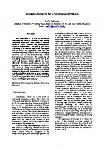
In this experiment, the Annealing Scheduler is compared to the Ad-Hoc scheduler to see which one produces better estimated schedules when given the same information. The list of available machines obtained from MDS and their characteristics obtained from NWS are cached, so that the scheduling is done using consistent information. The experimental testbed consisted of x86 CPUS running Linux; there were 3 machines from the University of Tennessee (UTK) TORC cluster (550 MHz PIII, 512 MB memory), 3 machines from the UTK MSC cluster (933 MHz PIII, 512 MB memory), and 9 machines from the University of Illinois (UIUC) OPUS cluster (450 MHz PII, 256 MB memory). The schedules that were generated were not actually run in this experiment since consistent machine information was required to test the schedulers, this information would have been stale by the time the runs were performed. The best schedules and their predicted execution times are shown in Figure 1. This testbed of 12 machines was not able to handle matrices of size 15000 or larger, so the largest problem that was scheduled was of size 14000. The annealing scheduler is usually able to find a schedule having a better estimated execution time than the Ad-Hoc scheduler. This trend is stronger for the larger matrix sizes. However, this estimated schedule depends on how accurately the Performance Model reflects reality.
3
1400 1000
Ad−Hoc Schedule Annealing Schedule
0
Estimated execution time (sec)
16: 17: 18: 19: 20: 21: 22:
600
8: 9: 10: 11: 12: 13: 14: 15:
200
1: 2: 3: 4: 5: 6: 7:
Algorithm 2: Scheduling using Simulated Annealing given N available machines from MDS with NWS information for each possible virtual machine size vmsize = 1...N do find all R machines having sufficient resources (i.e. free memory) if number of machines with sufficient resources R < vmsize then continue to next vmsize else {below we select best vmsize machines from R using Simulated Annealing} create an initial schedule using random n from the R eligible machines evaluate the Performance Model on the n selected machines using the dynamic NWS information repeat {at each temperature} for a number of steps, breaking for loop if energy stabilizes do perturb the schedule randomly, remove a machine, add another machine, and swap their order evaluate the Performance Model on the new schedule if energy (execution time) is decreased then accept new schedule unconditionally else accept new schedule if a random number < exp(−dE/kT ) [Metropolis step] end if end for decrease temperature until energy does not change or temperature is at minimum end if end for
1000
3000
5000
7000
9000
11000
13000
Size of matrices (N)
Figure 1: Estimated execution times for Simulated Annealing and Ad-Hoc schedules using static network information
4
3.2
Accuracy of the Generated Schedules
800 200
400
600
Ad−Hoc Schedule (estimated time) Annealing Schedule (estimated time)
0
Estimated Execution Time (sec)
In this experiment we want to determine how accurately the estimated execution time matches the actual execution time for the two schedulers. The difficulty is that the estimated schedules measure the accuracy of the Performance Model far more than the accuracy of the Scheduler. However, since the same Performance Model is used for both the Simulated Annealing scheduler as well as the Ad-Hoc scheduler, the comparison of the two schedulers shows how well they perform given the current Performance Model. If the Performance Model is not correct, we expect that the Ad-Hoc scheduler will perform somewhat better than the Simulated Annealing scheduler, since it includes some implicit knowledge of the application and the environment. For example, the Ad-Hoc greedy scheduler uses bandwidth as a major factor for ordering its selection of machines and generating a good schedule for the ScaLAPACK example. Also, it assumes that it is better to use machines within a cluster (having high connectivity) before using remote machines. These assumptions, though valid for the ScaLAPACK application, may not be valid in all cases. The Simulated Annealing scheduler is application agnostic; it creates the schedule without any knowledge of the application. The scheduler depends purely on the Performance Model, so if the Performance Model is accurate, the annealing scheduler will return accurate results. For this experiment, 25 machines from three Linux clusters at the were used as the testbed. Nine machines were from the UTK/TORC cluster (550 MHz PIII, 512 MB memory), 8 machines were from the UTK/MSC cluster (933 MHz PIII, 512 MB memory), and 8 machines were from the UIUC/OPUS cluster (450 MHz PII, 256 MB memory) . Figure 2 shows that estimated execution times for the runs using dynamic network (NWS) information. The difference
1000
3000
5000
7000
9000
11000
13000
Size of matrices (N)
Figure 2: Estimated execution time for the Ad-Hoc and Simulated Annealing schedules using dynamic network information between the estimated execution times for the two scheduling techniques is not as dramatic as in Figure 1, however, these measurements were taken at different times and under different network and load conditions, and the Ad-Hoc scheduler did not get caught in a bad local minima in this example as it did in Figure 1. Figure 3 shows the measured execution time when the generated schedules were run, and here we see that the measured times are generally larger than the estimated times. This exposes a problem with the current Performance Model, which does not properly 5
800 600 400 200 0
Measured Execution Time (sec)
Ad−Hoc Schedule (measured time) Annealing Schedule (measured time)
1000
3000
5000
7000
9000
11000
13000
Size of matrices (N)
Figure 3: Measured execution time for the Ad-Hoc and Simulated Annealing schedules using dynamic network information
6
2.5
account for the communication costs. The Simulated Annealing schedule generally takes a little less time than the Ad-Hoc schedule, however this trend is not totally consistent. Figure 4 shows the ratio of the measured execution time to the estimated execution time. If the Performance Model
●
Ad−Hoc Scheduler (measured/estimated) Annealing Scheduler (measured/estimated)
2.0
● ●
1.5
●
●
●
● ●
●
●
● ●
● ●
1.0
Ratio (measured/estimated)
●
2000
4000
6000
8000
10000
12000
14000
Matrix size (N)
Figure 4: Accuracy of Simulated Annealing and Ad-Hoc scheduling shown as ratio of measured execution time to estimated execution time was fully accurate and execution environment was perfectly known, the ideal ratio in Figure 4 would be a 1.0 across all the matrix sizes. However, both the schedulers differ substantially from the ideal, implying that the Performance Model is not estimating the time required for execution accurately for a distributed set of machines. There could be several reasons why this is happening, however the current belief is that the Performance Model does not properly account for the communication costs.
3.3
Overhead of the Scheduling Strategies
The Ad-Hoc scheduler has very little overhead associated with it. The number of times it has to evaluate the Performance Model for different machine configurations is at most (number of clusters × total number of available machines). This takes a negligible amount of time given the size of the current testbeds. The Simulated Annealing scheduler is has a higher overhead; however, it is still relatively small in comparison to the time required for most of the problems that would solved in a Grid environment. The time taken by simulated annealing is dependent on some of algorithm parameters, like the temperature reduction schedule and the desired number of iterations at each temperature, as well as the size of the space that is being searched. In our experiments, when the testbed consists of 38 machines, we got the maximum overhead of 57 seconds from the Simulated Annealing scheduling process (on a 500MHz PIII machine). This is still relatively small compared to execution time for most of the ScaLAPACK problems.
7
4
Future Research
Firstly, the Performance Model needs to be examined, to see if it can be improved. Also, the performance of the schedulers has to be verified on larger testbeds. In order to construct large, repeatable experiments, a simulation environment designed to examine application scheduling on the Grid such as SimGrid [7] could be used. Additional scheduling algorithms (using non-linear programming techniques, genetic algorithms, etc.) should also be evaluated. A possible improvement to the scheduling process might be to combine the Ad-Hoc and Simulated Annealing schedulers. The Ad-Hoc scheduler could be used to determine the approximate space where the optimal solution can be found (e.g., returning the approximate number N of machines to be used), and the Annealing Scheduler could be used to search that space more thoroughly (e.g., search using N − 1, N, N + 1 machines). This would combine the speed of the Ad-Hoc approach and retain elements of the global search process.
5
Summary
The Simulated Annealing scheduler generates schedules that have a better estimated execution time than those returned by the Ad-Hoc greedy scheduler. This is because the Simulated Annealing scheduler can avoid some of the local minima that are not anticipated in the ordering imposed in the Ad-Hoc techniques greedy search. When the generated schedules are actually executed, the measured execution time for the Annealing Scheduler is approximately the same or just a little better than the Ad-Hoc scheduler. Also, the measured execution time is sufficiently different from the estimated execution time that we need to re-examine the Performance Model being used.
References [1] D. Abramson, J. Giddy, and L. Kotler. High Performance Parametric Modeling with Nimrod/G: Killer Application for the Global Grid? In Proceedings of the 14th International Conference on Parallel and Distributed Processing Symposium (IPDPS-00), pages 520–528, Los Alamitos, May 1–5 2000. IEEE. [2] A. H. Alhusaini, C. S. Raghavendra, and V. K. Prasanna. Run-Time adaptation with resource Co-Allocation for Grid environments. In Proceedings of the 15th International Parallel & Distributed Processing Symposium (IPDPS-01), pages 87–87, Los Alamitos, CA, April 23–27 2001. IEEE Computer Society. [3] Francine Berman. High-performance schedulers. In Ian Foster and Carl Kesselman, editors, The Grid: Blueprint for a New Computing Infrastructure, pages 279–309. Morgan Kaufmann, San Francisco, CA, 1999. [4] Francine Berman, Andrew Chien, Keith Cooper, Jack Dongarra, Ian Foster, Dennis Gannon, Lennart Johnsson, Ken Kennedy, Carl Kesselman, John Mellor-Crummey, Dan Reed, Linda Torczon, and Rich Wolski. The GrADS Project: Software support for high-level Grid application development. The International Journal of High Performance Computing Applications, 15(4):327–344, November 2001. [5] Francine D. Berman, Rich Wolski, Silvia Figueira, Jennifer Schopf, and Gary Shao. Application-level scheduling on distributed heterogeneous networks. In ACM, editor, Supercomputing ’96 Conference Proceedings: November 17–22, Pittsburgh, PA, New York, NY 10036, USA and 1109 Spring Street, Suite 300, Silver Spring, MD 20910, USA, 1996. ACM Press and IEEE Computer Society Press. [6] L. S. Blackford, J. Choi, A. Cleary, E. D’Azevedo, J. Demmel, I. Dhillon, J. Dongarra, S. Hammarling, G. Henry, A. Petitet, K. Stanley, D. Walker, and R. C. Whaley. ScaLAPACK: a linear algebra library for message-passing computers. In Proceedings of the Eighth SIAM Conference on Parallel Processing for Scientific Computing (Minneapolis, MN, 1997), page 15 (electronic), Philadelphia, PA, USA, 1997. Society for Industrial and Applied Mathematics. [7] Henri Casanova. Simgrid: A Toolkit for the Simulation of Application Scheduling. In Proceedings of the First IEEE/ACM International Symposium on Cluster Computing and the Grid (CCGrid 2001), Brisbane, Australia, May 15–18 2001.
8
[8] Holly Dail. A Modular Framework for Adaptive Scheduling in Grid Application Development Environments. Master’s thesis, University of California, San Diego, 2002. [9] I. Foster and C. Kesselman. Globus: A Metacomputing Infrastructure Toolkit. The International Journal of Supercomputer Applications and High Performance Computing, 11(2):115–128, Summer 1997. [10] Ian Foster and Carl Kesselman. The Globus Toolkit. In Ian Foster and Carl Kesselman, editors, The Grid: Blueprint for a New Computing Infrastructure, pages 259–278. Morgan Kaufmann, San Francisco, CA, 1999. Chap. 11. [11] Andrew S. Grimshaw, William A. Wulf, and the Legion team. The Legion Vision of a Worldwide Virtual Computer. Communications of the ACM, 40(1):39–45, January 1997. [12] Scott Kirkpatrick. Optimization by Simulated Annealing: Quantitative Studies. Journal of Statistical Physics, 34(5-6):975–986, 1984. [13] N. Metropolis, A. W. Rosenbluth, M. N. Rosenbluth, A. H. Teller, and E. Teller. Equations of state calculations by fast computing machines. J. Chem. Phys., 21:1087–1091, 1953. [14] Antoine Petitet, Susan Blackford, Jack Dongarra, Brett Ellis, Graham Fagg, Kenneth Roche, and Sathish Vadhiyar. Numerical libraries and the Grid. The International Journal of High Performance Computing Applications, 15(4):359–374, November 2001. [15] Tindell, Burns, and Wellings. Allocating hard real-time tasks: An NP-hard problem made easy. RTSYSTS: Real-Time Systems, 4, 1992. [16] J Ullman. NP-Complete Scheduling Problems. Journal of Computer and System Sciences, 10:384–393, 1975. [17] J. Weissman and X. Zhao. Scheduling Parallel Applications in Distributed Networks. Journal of Cluster Computing, pages 109–118, 1998. [18] Jon B. Weissman. Prophet: automated scheduling of SPMD programs in workstation networks. Concurrency: Practice and Experience, 11(6):301–321, May 1999. [19] Rich Wolski, Neil T. Spring, and Jim Hayes. The Network Weather Service: a Distributed Resource Performance Forecasting Service for Metacomputing. Future Generation Computer Systems, 15(5–6):757–768, October 1999.
9