tion of counterexamples demonstrating that a system does not satisfy ....
executions relevant for analysis or to generate them from a counterexample. Jin,
Ravi ...
What Went Wrong: Explaining Counterexamples Alex Groce1 and Willem Visser2 1
2
Department of Computer Science Carnegie Mellon University Pittsburgh, PA, 15213 RIACS/NASA Ames Research Center Moffett Field, CA 94035-1000
Abstract. One of the chief advantages of model checking is the production of counterexamples demonstrating that a system does not satisfy a specification. However, it may require a great deal of human effort to extract the essence of an error from even a detailed source-level trace of a failing run. We use an automated method for finding multiple versions of an error (and similar executions that do not produce an error), and analyze these executions to produce a more succinct description of the key elements of the error. The description produced includes identification of portions of the source code crucial to distinguishing failing and succeeding runs, differences in invariants between failing and nonfailing runs, and information on the necessary changes in scheduling and environmental actions needed to cause successful runs to fail.
1
Introduction
In model checking [4], algorithms are used to systematically determine whether a system satisfies a specification. One of the major advantages of model checking in comparison to such methods as theorem proving is the production of a counterexample that provides a detailed example of how the system violates the specification when verification fails. However, even a detailed trace of how a system violates a specification may not provide enough information to easily understand (much less remedy) the problem with the system. Model checking is particularly effective at finding subtle errors that can elude traditional testing, but consequently the errors are also difficult to understand, especially from a single error trace. Furthermore, when the model of the system is in any sense abstracted from the real implementation, simply determining whether an error is indeed a fault in the system or merely a consequence of modeling assumptions or incorrect specification can be quite difficult. We attempt to extract more information from a single counterexample produced by model checking in order to facilitate understanding of errors in a system (or problems with the specification of a system). We focus in this work on finite executions demonstrating violation of safety properties (e.g. assertion violations, uncaught exceptions, and deadlocks) in Java programs. The key to this approach is to first define (and then find) multiple variations on a single counterexample
(other versions of the “same” error). From this definition naturally arises that of a set of executions that are variations in which the error does not occur. We call the first set of executions negatives and the second set positives. Analysis of the common features of each set and the differences between the sets may yield a more useful feedback than reading (only) the original counterexample. One approach to analysis would be to define the negatives as all executions that reach a particular error state (all deadlocks, all assertion violations, etc.). This definition has major drawbacks. A complex concurrent program, for example, may have many deadlocks that have different causes. Attempts to extract any common features from the negatives are likely to fail or be computationally expensive (for example, requiring clustering) in this case. The second problem is that positives would presumably be any executions not ending in the error state, again making comparison difficult. In software, at least, we usually think of errors as occurring at a particular place—e.g., a deadlock at a particular synchronization, or a failure of a particular assertion or array-out-of-bounds error at a particular point in the source code. We define negatives, therefore, as executions that not only end in the same error state, but that reach it from the same control location. Rather than analyzing all deadlocks, our definition focuses analysis on deadlocks that occur after the same attempt to acquire a lock, for example. We believe that our definition formally captures a simplified version of the programmer’s notion of “the same error.” Positives are the executions that pass through that control location without proceeding to an error state. We present three different analyses that can be automatically extracted from a set of negatives and positives. The first is based on the transitions appearing in the set. The second is based on data invariants over the executions. The last analysis discovers minimal transformations between negatives and positives. This paper is organized as follows: in Section 2 we discuss related work. The definitions of negative and positive executions are then formalized in Section 3, followed by a presentation of an algorithm for generating executions to analyze in Section 4. The various analyses currently applied and their implementations are discussed in Section 5 and Section 6, respectively. We then present experimental results in Section 7, followed by conclusions and future work.
2
Related Work
The most closely related work to ours is that of Ball, Naik, and Rajamani [1]. They find successful paths to the control location at which an error is discovered in order to find the cause of the error. Once a cause is discovered, they model check a restricted model in which the system is restricted from executing the causal transitions to discover if other causes for the error are possible. The analysis provided is similar to our transition analysis; no method analogous to invariant or transformation analysis is provided, nor are concurrent programs analyzed. This error analysis has been implemented for the SLAM [2] tool. Sharygina and Peled [13] propose the notion of the neighborhood of a counterexample and suggest that an exploration of this region may be useful in
understanding an error. However, the exploration, while aided by a testing tool, is essentially manual and offers no automatic analysis. No formal notion of other versions of the same error is presented. Dodoo, Donovan, Lin and Ernst [5] use the Daikon invariant detector to discover differences in invariants between passing and failing test cases, but propose no means to restrict the cases to similar executions relevant for analysis or to generate them from a counterexample. Jin, Ravi and Somenzi [11] proceed from the same starting point of analyzing counterexamples produced by a model checker. Their goal is also similar: providing additional feedback in addition to the original counterexample in order to deal with the complexity of errors. Fate and free will are terms in a game in which a counterexample is broken into parts depending on whether the environment (attempting to force the system into an error state) or the system (attempting to avoid error) controls it. This approach produces a different kind of explanation (an alternation of fated and free segments). The work of Andreas Zeller was also an important influence on this work. Delta debugging is a technique for minimizing error trails that works by conducting a modified binary search between a failing run and a succeeding run of a program [17]. Zeller has extended this notion to other approaches to automatic debugging, including modifying portions of a program’s state to isolate causeeffect chains [16] and discovering the minimal difference in thread scheduling necessary to produce a concurrency-based error [3]. Our computation of transformations between positive and negative executions was inspired by this approach, particularly in that we look for minimal transformations.
3
Definitions
The crucial definitions are those of negatives and positives, the two classes of executions we use in our analysis. While manual exploration of paths near a counterexample can be useful [13], a formal definition of a variation on a counterexample is necessary before proceeding to the more fruitful approach of automatic generation and analysis of relevant executions. Intuitively, we examine the full set of finite executions in which the program reaches the control location immediately proceeding the error state. A labeled transition system (LTS) is a 4-tuple hS, S0 , Act, T i, where S is a finite non-empty set of states, S0 ⊂ S is the set of initial states, Act is the set of actions, and T ⊂ S × Act × S is the transition relation. We assume that S contains a distinguished set of error states (with no outgoing transitions), Π = {π0 , · · · , πn } (representing, e.g. deadlock, assertion violation, uncaught exception. . . ). We also introduce a set C of control locations and a set D of data valuations, such that S = (C ×D)∪Π, and introduce partial projection functions α c : S → C and d : S → D. We write s −→ s0 as shorthand for (s, α, s0 ) ∈ T . α1 α2 A finite transition sequence from s0 ∈ S is a sequence t = s0 −→ s1 −→ αk · · · −→ sk , where 0 < k < ∞. We refer to k as the length of t, also denoted αk α2 α1 · · · −→ sk s1 −→ by |t|. We say that a finite transition sequence t = s0 −→ α0
α0
α0 0
1 2 k is a prefix of a finite transition sequence t0 = s00 −→ s01 −→ · · · −→ sk0 if
0 < k < k 0 and ∀i ≤ k . (i ≥ 0 ⇒ si = s0i ) ∧ (i > 0 ⇒ αi = αi0 ). We say that αk α1 α2 a finite transition sequence t = s0 −→ s1 −→ · · · −→ sk is a control suffix of α0
α0 0
α0
1 2 k a finite transition sequence t0 = s00 −→ s01 −→ · · · −→ sk0 iff 0 < k < k 0 and 0 ∀i ≤ k . (i ≥ 0 ⇒ c(sk−i ) = c(sk0 −i )) ∧ (i > 0 ⇒ αk−i = αk0 0 −i ). We also define the empty transition sequence, emp as consisting of no states or actions, where |emp| = 0. We consider the class of counterexamples that are finite transition sequences αk α1 α2 from s0 ∈ S0 . Given an initial counterexample t = s0 −→ s1 −→ · · · −→ sk , where sk ∈ Π, we define a negative as an execution that results in the same error state from the same control location (the original counterexample is itself a negative). Formally: Definition: Negative: A negative (with respect to a particular t, as noted
α0
α0
α0 0
1 2 k · · · −→ s0k0 , above) is a finite transition sequence from s00 ∈ S0 , t0 = s00 −→ s01 −→ 0 where 0 < k < ∞, such that:
1. c(sk−1 ) = c(s0k0 −1 ) ∧ αk = αk0 0 and 2. sk = s0k0 . We then define neg(t) as the set of all negatives with respect to a counterexample t. The original counterexample itself is one such negative, and is used as such in all analyses. Definition: Positive: A positive (with respect to t) is a finite transition α0
α0
α0 0
1 2 k sequence from s00 ∈ S0 , t0 = s00 −→ s01 −→ · · · −→ s0k0 , where 0 < k 0 < ∞ such that:
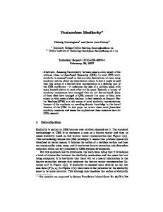
1. c(sk−1 ) = c(s0k0 −1 ) ∧ αk = αk0 0 , 2. s0k0 ∈ 6 Π, and 3. ∀t00 ∈ neg(t) . t0 is not a prefix of t00 . We define pos(t) as the set of all positives with respect to a counterexample t, and var(t) as neg(t) ∪ pos(t), the set of all variations on the original counterexample. We will henceforth refer to neg and pos, omitting the implied parameterization with respect to t. Figure 1 shows an example. The numbers inside states indicate the control location of the state, c(s), and the letters beside the arrows are the labels of actions (in this case drawn from the alphabet {a, b}). The original counterexample ends in the state A ∈ Π, indicating an assertion violation. The negative shown takes a different sequence of actions but also passes through the control location 3, takes an a action, and transitions to the error state A. The positive reaches control location 3 but in a data state such that taking an a action transitions to a non-error state. These basic definitions, however, give rise to certain difficulties in practice. First, the set of negatives is potentially infinite, as is the set of positives. On the other hand, the set of positives may be empty, as an error in a reactive system is often reachable from any other state. For reasons of tractability we generate and analyze subsets of the negatives and positives. When only a subset of negatives
0
0
0 a
a 1
1
a
b 4
2
5
A
a 3 a
a
a Counterexample
b 5
b
b 3
b 2
4
3 a A
Positive
Negative
Fig. 1. A counterexample, a negative, and a positive.
are known the third condition in the definition of positives cannot be checked; we therefore replace it with the weaker requirement that t0 not be a prefix of any negative we generate.
4
Generation of Positives and Negatives
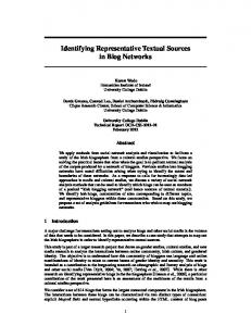
The algorithm for generating a subset of the negatives (and a set of potential positives, per the modified prefix condition) uses a model checker to explore backwards from the original counterexample. We describe an explicit state algorithm, but are investigating a SAT-based approach. We assume that the model checker (M C) can be called as a function during generation with an initial state s from which to begin exploration, a maximum search depth d, a control state to match c, an error state π, and a visited set v. The model checker returns two (possibly empty) sets: n (negatives) and p (potential positives) and a new visited set v 0 . The check for whether a state is the last in a positive or negative is a simple safety property relying only on a state’s control location and the preceeding control location and action (see the above definitions), and should not pose difficulties. Removal of prefixes of negatives is done in a final stage and need not be taken into account by the model checker. The generation algorithm (Figure 2) takes as input an initial counterexample αk α1 α2 t = s0 −→ s1 −→ · · · −→ sk and a search depth d. The model checking algorithm used is not specified, but we make a few assumptions about its behavior. If a depth limit is not given each call to the model checker will only terminate upon exploring the full reachable state space from si , so we assume that the model checker allows the use of depth limits. We also require that the model checker be able to report multiple counterexamples (paths to all states satisfying the properties for defining negatives and positives). Both of these assumptions can easily be met by various explicit state model checkers—e.g. SPIN supports depth limits as well as multiple counterex-
generate (t, d) v := neg := pos := ∅ i := k − 1 while i >= 0 (n, p, v) := M C(si , t, d, v) neg := neg ∪ n pos := pos ∪ p i := i − 1 for all t ∈ pos for all t0 ∈ neg if t is a prefix of t0 pos := pos \ t return (neg, pos)
Fig. 2. Algorithm for generation of negatives and positives.
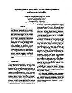
amples. The counterexamples can be split into negatives and positives after being returned, if necessary. To provide more negatives and positives to analyze we also propose one alteration to the internal behavior of the model checker. When the depth limit is reached, we attempt to extend the execution to match the original counterexample. This causes the depth limit to behave as an edit-distance from the original counterexample: negatives and positives may deviate from the original execution for a number of actions limited by d. The algorithm for extension, proceeding from a state s at depth i is given in Figure 3. Briefly, the algorithm checks the state at which exploration terminates due to depth limiting to see if it matches control location with any state further along the original counterexample. For all matches, the actions taken in the original counterexample are repeated if enabled in order to reach either a negative or a positive. The extension algorithm is depth-first, but can be integrated into both breadth-first and heuristic-based model checking algorithms.
j := i while j < k if c(sj ) = c(s) s0 := s l := j + 1 broken := f alse while l < k ∧ ¬ broken αl if ∃ s00 . s0 −→ s00 ∧ c(s00 ) = c(sl ) ∧ s00 6∈ v 0 00 s := s else broken := true l := l + 1 if ¬ broken αk if s0 −→ s00 if s00 ∈ Π add transition sequence to s00 to current set of negatives else add transition sequence to s00 to current set of positives j := j + 1
Fig. 3. Algorithm for extension.
We use neg and pos below to denote the sets returned by this generation algorithm, not the true complete sets of negatives and positives.
5
Analysis of Variations
Once the negatives and positives have been generated, it remains to produce from them useful feedback for the user. Even without such analysis, the traces may prove useful, but our experience shows that even tightly limited searches will produce large numbers of traces that are as difficult to understand in isolation as the original counterexample. It is not the traces in and of themselves that provide leverage in understanding the error; any negative could have generally been substituted for the original counterexample, and a positive simply shows an instance of the program reaching a control location without error. 5.1
Transition Analysis
The various analyses we employ are designed to characterize (1) the common elements of negatives/positives and (2) the difference between negatives and positives. For this analysis, we examine the presence of transitions in the executions in each set. In particular we compute sets containing projected transitions, pairs hc, αi, where c ∈ C is a control location and α ∈ Act is an action. We say that αk α1 α2 the finite transition sequence t = s0 −→ s1 −→ · · · −→ sk contains hc, αi iff ∃n < k . c(sn ) = c ∧ αn+1 = α. The analysis below can also be computed using only projected control locations, ignoring actions (or also projecting on some portion of a composite action, when this is possible). Transition Analysis Set Definition trans(neg) hc, αi|∃t ∈ neg . t contains hc, αi trans(pos) hc, αi|∃t ∈ pos . t contains hc, αi all(neg) hc, αi|∀t ∈ neg . t contains hc, αi all(pos) hc, αi|∀t ∈ pos . t contains hc, αi only(neg) trans(neg)\trans(pos) only(pos) trans(pos)\trans(neg) cause(neg) all(neg) ∩ only(neg) cause(pos) all(pos) ∩ only(pos)
Table 1. Transition analysis set definitions.
In transition analysis, we compute a number of sets of transitions, listed in Table 1. trans(neg) and trans(pos) are complete sets of all transitions appearing in negatives and positives, respectively. The sets all(neg) and all(pos) (transitions appearing in all negatives or positives) are reported directly to the user. These may be sufficient to explain an error, either by indicating that certain code is faulty or that execution of certain code prevents the error from appearing. Also reported to the user are the transitions appearing only in negatives/positives, only(neg) and only(pos). Finally, potentially causal transition sets are reported.
The rationale for computing causal sets is that in many cases all(neg) and all(pos) will contain a number of common elements, due to common initialization code and aspects of execution unrelated to the error. only(neg) and only(pos) may also be large sets if the error induces differing behavior in the system before the point at which the error is detected. When non-empty, cause(neg) and cause(pos) denote sets that are potentially much smaller and denote precisely the common behavior that differentiates the negative and positive sets. The error cause localization algorithm used in SLAM is comparable to reporting either cause(neg) or only(neg), as SLAM analyzes one error trace at a time [1].
1 2 3 4 5 6 7 8 9 10 11
int got lock = 0; do { if (Verify.chooseBool ()) { lock (); got lock++; } if (got lock != 0) { unlock (); } got lock--; } while (Verify.chooseBool ());
public static void lock () { Verify.assertTrue (LOCK == 0); LOCK = 1; }
public static void unlock () { Verify.assertTrue (LOCK == 1); LOCK = 0; }
Fig. 4. Example 1.
Example of Transition Analysis The Java code in Figure 4 (adapted from a BLAST example [10]) calls lock and unlock methods that assert that the lock is not held and the lock is held, respectively. Verify.chooseBool () indicates a nondeterministic choice between true and false (see Section 6). The bug (line 10 should be inside the scope of the if starting at line 7) can appear as a violation of either the lock or unlock assertion. Depth-30 analysis from a counterexample F in which the unlock assertion is violated (1 −→ 2 −→ 3 −→ 7 −→ 10 −→ T F 11 −→ 3 −→ 7 −→ 8 −→ A) discovers two positives and two negatives. Transition Analysis Set Elements all(neg) {1, 2, h3, F i, 7, 8, 10, h11, T i} all(pos) {1, 2, h3, T i, 4, 5, 7, 8} only(neg) {h3, F i, 10, h11, T i} only(pos) ∅ cause(neg) {h3, F i, 10, h11, T i} cause(pos) ∅
Table 2. Transition analysis example results.
In this case cause(neg) is unchanged by our use of the weaker prefix constraint for positives (there are no real positives in this program: the error can occur in an extension of every trace ending at line 8). Here cause(neg) notes
the key points of the unlocking error: the system chooses not to lock (h3, F i), which means that the decrement of got lock (10) is incorrect (the lock’s status has not been changed this time through the loop). Reiterating the loop (h11, T i) makes it possible to try to unlock when the lock has not been acquired. 5.2
Invariant Analysis
Transition analysis is useful when the control flow or action choices independent of ordering are sufficient to explain an error. However, the same actions from the same control locations may be present in both negatives and positives; it may be that the choice of an action with respect to d(s) rather than c(s) is crucial. A set-based approach projected on d(s) rather than c(s) faces the problem that only certain data values are likely to be relevant, rather than the full state. Instead, we compute data invariants over the negatives and compare them to the invariants over the positives. Specifically, the user may choose certain control locations as instrumentation points. The value of d(s) (or some projection over certain variables of the data state) is recorded for each transition sequence every time the control flow reaches the instrumentation locations. We then compute invariants using Daikon [6] (see Section 6 for details) with respect to each of the instrumentation points over all negatives and all positives. The invariants for negatives are then compared to the invariants for positives, and the user is presented with this difference. Daikon’s analysis is dynamic and thus unsound; however, the invariants reported over a set of traces (which is precisely what we are concerned with here) are always correct for those traces. Choosing instrumentation points and how deeply to instrument (by default all local primitive-typed variables, but JPF can also report on object fields and other frames) is not automated and must be guided by user knowledge the other analyses. int a = Verify.choose(4); int b = Verify.choose(4); // nondeterministic 0-4 int c = Verify.choose(4); int d = Verify.choose(4); // nondeterministic 0-4 int temp = 0; Verify.instrumentPoint("pre-sort"); if (a > b) { temp = b; b = a; a = temp; } // Swap if (b > c) { temp = c; c = b; b = temp; } // Swap if (c > d) { temp = d; d = c; c = temp; } // Swap if (b > c) { temp = c; c = b; b = temp; } // Swap Verify.instrumentPoint("post-sort"); Verify.assertTrue((a = 0 a’ >= 1 a’ b’ a’ temp
Table 3. Invariant analysis example results.
We observe from the negative invariants that a’ may be greater than b’. Because invariant analysis is complete over the negative and positive runs, the absence of an a’ k − |u| then tp = emp. α0k
+1
t 5. tn = s0kt −→ · · · sk0 −|u| If kt > k 0 − |u| then tn = emp.
The last two definitions select the diverging portions of t and t0 as the positive (tp ) and negative (tn ) portions of the transformation (see Figure 6). When S0 contains a single state, there will exist a minimal transformation for every pair in pos × neg. Sorting this set by a metric of transformation size (|tp | + |tn | is one reasonable choice, though this ignores similarities within the transformation) yields a description of increasingly complex ways to cause a successful execution to fail. This set (along with the associated positive(s) and negative(s) for each transformation) can aid understanding of aspects of an error (such as timing or threading issues) that are not expressible by either transition
or invariant analysis. For example, if a positive can be transformed into a negative by changing actions that represent thread/process scheduling choices only, an error can be immediately classified as a concurrency problem. Additionally, we reapply the transition analysis with the values of tp replacing pos and the values of tn replacing neg. This may yield causal transitions when none are discovered by the first analysis (because the context in which the transitions are executed is important). Returning to the example in Figure 4, running transformation analysis gives T F us two distinct minimal transformations: (3 −→ 4 −→ 5 −→ 7) → (3 −→ 7 −→ T F T F 10 −→ 11 −→ 3 −→ 7) and (3 −→ 4 −→ 5 −→ 7) → (3 −→ 7 −→ 10 −→ T T T F T 11 −→ 3 −→ 4 −→ 5 −→ 7 −→ 10 −→ 11 −→ 3 −→ 7 −→ 8 −→ 10 −→ 11 −→ F 3 −→ 7). The first of these can be read as “the error will occur in this execution if, rather than choosing to acquire the lock (tp ), the system, in a state where get lock == 0, decrements get lock, then chooses to loop around and again chooses not to acquire the lock (tn ).” The second example produces the negative in which the lock is acquired once—only on the second iteration through the loop does get lock’s value become incorrect with respect to the guard in line 7.
6
Implementation
We implemented our algorithm for generating and analyzing variations inside the Java PathFinder model checker [15]. Java PathFinder (JPF) is an explicit state on-the-fly model checker that takes compiled Java programs (i.e. bytecode class-files) and analyzes all paths through the program for deadlock, assertion violations and linear time temporal logic (LTL) properties. In this implementation we only consider safety properties. We hope to consider the analysis of LTL counterexamples in future work. Actions of an environment not under the control of the Java program are represented in JPF as nondeterministic choices, introduced with special Verify.chooseBool() or Verify.choose(int i) calls which are trapped by the model checker. For example, Verify.choose(2) will nondeterministically return a value in the range 0–2, inclusive. In terms of the LTS model used above, Act = (t×n), where t is a non-negative integer identifying the thread executing in the step, and n is either a non-negative integer indicating a nondeterministic choice resulting from a Verify call (or -1, indicating no such call was made). Π is the set {deadlock, assertion, exception} indicating that there is a deadlock, an assertion was violated, or that an uncaught exception was raised. States are the various states of the JVM (including states for each member of Π). c(s) returns a set of control locations (bytecode positions), one for each thread in the current state, allowing for further projection of the control location along each thread. Our implementation of error explanation makes use of JPF’s various search capabilities to provide a wide range of possible searches during the generation of variations, including heuristic searches [8]. We have added the ability to produce Daikon [6] trace files to JPF. Daikon is a tool that takes trace files generated by instrumented code and discovers
invariants over the set of traces. We use Daikon for invariant analysis. The other analysis techniques are implemented inside JPF. In JPF, all executions start from the same initial state of the JVM, so the full transformation set always exists. For transition analysis JPF allows various projections on actions, such as ignoring nondeterministic choice or selected thread, as well as analysis based only on control location. In the JPF implementation, we universally use, rather than the c(s) defined above, a projection that produces only the control location of the thread that is executed from a state (c(s, α)), an improvement in almost all cases where there are well-defined control locations for threads or processes.
7
Experimental Results
We applied error explanation to determine the cause of a subtle error in an early version of the DEOS real-time operating system used by Honeywell in small business aircraft. We studied this system originally [12] knowing only that an error was present. When we found the error it took us hours to determine that the counterexample given was non-spurious (a time abstraction was used) and showed the error sought. Given this experience and the fact that the DEOS error is very subtle we believed this to be a good test of the error explanation approach. We analyzed a 1500 line Java translation of (a slice of) the original C++ system. DEOS is a real-time operating system based on rate-monotonic scheduling that allows user-threads to make kernel calls during their execution; for example, they can yield the CPU by making a WaitUntilNextPeriod call or remove themselves by making a Delete call. Since threads can have different priority they can be interrupted by a higher priority thread when a SystemTick happens (indicating a new scheduling period starting), or they can use up all their allotted time, indicated by a TimerInterrupt. We were checking a safety property asserting time-partitioning—a thread always gets the amount of time it asked for—checked whenever a new thread is to be scheduled. JPF found the original error in 52 seconds (on a 2.2Ghz Pentium with 2GB of memory), and then spent another 102 seconds performing a depth-limit 30 analysis (finding 131 variations on the error in the process). The resulting output indicated the following key points: – The Delete call is present in all negatives, but also in some positives. – The shortest transformations from positive runs to negatives are: • replacing a WaitUntilNextPeriod with a Delete call; • inserting a TimerInterrupt and a SystemTick before a Delete call. This shows that the Delete call is essential to the error, but only in specific circumstances. This matches the cause of the known error, where a Delete call is performed after a specific amount of time has elapsed. Note that making a Delete call by itself is not sufficient to cause the error, since there are positives containing this call. It took approximately 15 minutes to analyze the output file produced from the error explanation to determine the cause.
One difficulty with the DEOS example is that we were already familiar with the code and the problem. We applied error analysis to a mode-confusion in an autopilot system [14]. In this case, a user unfamiliar with the code and error was able to describe (relying primarily on the transformation analysis) the problem and generalize to the sequences of actions in which it arises. We also applied error analysis to concurrency errors such as those in the Remote Agent [9] and the executive planner of a Mars planetary rover. Transformation analysis identified concurrency errors in both cases and showed how minimal scheduling changes resulted in error.
8
Conclusions and Future Work
We propose definitions for two kinds of variations on a counterexample discovered during model checking and present an algorithm for generating a subset of these variations. These successful and failing executions are then used by various analysis routines to provide users with a variety of indications as to the important aspects of the original counterexample. The analyses suggested provide feedback on (1) control locations and actions key to the error (2) data invariant differences key to the error and (3) means of transforming successful executions into counterexamples. While further experiments are needed, our results demonstrate that this analysis can be useful in understanding complex errors. An important feature of our approach is that we do not have to assume we can compute the full set of reachable states in order to perform analysis—unlike in the related approaches of [1] and [11]. In our experience, when a counterexample can be found, error explanation to a useful search depth is also feasible. In particular, we could find and explain concurrency errors in the Mars rover (8K lines of code with a complicated control structure involving seven threads and complicated exception handling) although it has a very large state space that cannot be fully explored by JPF. Note that since we cannot always explore the complete state space of a system, we might not be able to show that an error is no longer present in a corrected system. In this case, however, we can use the set of negatives for the original counterexample during regression testing. The exploration algorithm used to generate negatives and positives can also be used to find a counterexample by searching “close to” a path the user suspects could lead to an error. As an example we used JPF’s race detection feature [15] to find race conditions in the Remote Agent (without finding any deadlocks or property violations), then fed the path to a race violation to the error explanation facility as the “counterexample” and found a property violation (a deadlock). The most important area of further research should be improving the methods of analysis both to provide more useful feedback and to do more automatic classification of errors. While the goal of routinely reporting “change line i in the following manner” is unlikely ever to be reached, we believe that better methods than the rudimentary ones presented here may exist. In particular, automatic analysis of the transformations between positives and negatives should be taken a step further than merely noting concurrency-only differences. Another possi-
bility is to generate from the negatives an automaton for an environment that avoids reproducing the error as in the work of Giannakopoulou, P˘as˘areanu, and Barringer [7]. It is possible that in some instances such an assumption might succinctly characterize the error, although as an assumption it would only be an approximation of the most general environment for the program.
References 1. T. Ball, M. Naik, and S. Rajamani. From Symptom to Cause: Localizing Errors in Counterexample Traces. In Principles of Programming Languages, 2003. 2. T. Ball and S. K. Rajamani. Automatically Validating Temporal Safety Properties of Interfaces. In SPIN Workshop on Model Checking of Software, pages 103–122, 2001. 3. J. Choi, and A. Zeller. Isolating Failure-Inducing Thread Schedules. In International Symposium on Software Testing and Analysis, 2002. 4. E. M. Clarke, O. Grumberg, and D. Peled. Model Checking. MIT Press, 2000. 5. N. Dodoo, A. Donovan, L. Lin and M. Ernst. Selecting Predicates for Implications in Program Analysis. http://pag.lcs.mit.edu/~mernst/pubs/ invariants-implications-abstract.html. March 16, 2000. Viewed: September 6th, 2002. 6. M. Ernst, J. Cockrell, W. Griswold and D. Notkin. Dynamically Discovering Likely Program Invariants to Support Program Evolution. In International Conference on Software Engineering, pages 213–224, 1999. 7. D. Giannakopoulou, C. P˘ as˘ areanu, and H. Barringer. Assumption Generation for Software Component Verification. In Automated Software Engineering, 2002. 8. A. Groce and W. Visser. Model Checking Java Programs using Structural Heuristics. In International Symposium on Software Testing and Analysis, 2002. 9. K. Havelund, M. Lowry, S. Park, C. Pecheur, J. Penix, W. Visser and J. White. Formal Analysis of the Remote Agent Before and After Flight. In Proceedings of the 5th NASA Langley Formal Methods Workshop, June 2000. 10. T. A. Henzinger, R. Jhala, R. Majumdar and G. Sutre. Lazy Abstraction. In ACM SIGPLAN-SIGACT Conference on Principles of Programming Languages, 2002. 11. H. Jin, K. Ravi and F. Somenzi. Fate and Free Will in Error Traces. In Tools and Algorithms for the Construction and Analysis of Systems, pages 445–458, 2002. 12. J. Penix, W. Visser, E. Engstrom, A. Larson and N. Weininger. Verification of Time Partitioning in the DEOS Scheduler Kernel. In International Conference on Software Engineering, pages 488–497, 2000. 13. N. Sharygina and D. Peled. A Combined Testing and Verification Approach for Software Reliability. In Formal Methods for Increasing Software Productivity, International Symposium of Formal Methods Europe, pages 611–628, 2001. 14. O. Tkachuk, G. Brat and W. Visser. Using Code Level Model Checking To Discover Automation Surprises. In Digital Avionics Systems Conference, Irvine CA, October 2002. 15. W. Visser, K. Havelund, G. Brat and S. Park. Model Checking Programs. In Automated Software Engineering (ASE), pages 3–11, 2000. 16. A. Zeller. Isolating Cause-Effect Chains from Computer Programs. In International Symposium on the Foundations of Software Engineering (FSE-10), 2002. 17. A. Zeller and R. Hildebrandt. Simplifying and Isolating Failure-Inducing Input. In IEEE Transactions on Software Engineering, 28(2), February 2002, pages 183–200.