Explanation Oriented Retrieval Dónal Doyle1, Pádraig Cunningham1, Derek Bridge2, Yusof Rahman1 1 Computer Science, Trinity College, Dublin 2, Ireland {Donal.Doyle, Padraig.Cunningham, Yusof.Rahman}@cs.tcd.ie 2 Computer Science, University College Cork, Cork, Ireland
[email protected]
Abstract. This paper is based on the observation that the nearest neighbour in a case-based prediction system may not be the best case to explain a prediction. This observation is based on the notion of a decision surface (i.e. class boundary) and the idea that cases located between the target case and the decision surface are more convincing as support for explanation. This motivates the idea of explanation utility, a metric that may be different to the similarity metric used for nearest neighbour retrieval. In this paper we present an explanation utility framework and present detailed examples of how it is used in two medical decision-support tasks. These examples show how this notion of explanation utility sometimes select cases other than the nearest neighbour for use in explanation and how these cases are more convincing as explanations.
1 Introduction This paper presents a framework for retrieving cases that will be effective for use in explanation. It is important to distinguish the type of explanation we have in mind from knowledge intensive explanation where the cases contain explanation structures [9,10]. Instead, this framework is concerned with knowledge light explanation where case descriptions are used in much the same way that examples are invoked for comparison in argument [6,8,10,11]. In this situation the most compelling example is not necessarily the most similar. For instance, if a decision is being made on whether to keep a sick 12 week old baby in hospital for observation, a similar example with a 14 week old baby that was kept in is more compelling than one with an 11 week old baby (based on the notion that younger babies are more likely to be kept in).1 The situation where the nearest neighbour might not be the best case to support an explanation arises when the nearest neighbour is further from the decision boundary than the target case. A case that lies between the target case and the decision boundary will be more useful for explanation. Several examples of this are presented in Section 4. In this paper we present a framework for case retrieval that captures this idea of explanation utility. We describe how this framework works and show several examples of how it can return better explanation cases than the similarity metric. 1
This is sometimes referred to as an a fortiori argument with which all parents will be familiar: the classic example is “How come Joe can stay up later than me when I am older than him?”.
An obvious question to ask is, why not use this explanation utility metric for classification as well as explanation? An investigation of this issue, presented in Section 5, shows that classification based on similarity is more accurate than classification based on our explanation utility metric. This supports our core hypothesis that the requirements for a framework for explanation are different to those for classification. The next section provides a brief overview of explanation in CBR before the details of the proposed explanation utility framework are described in section 3. Some examples of the explanation utility framework in action are presented in section 4 and the evaluation of the framework as a mechanism for classification (compared with classification based on similarity) is presented in section 5.
2 Explanation in Case Based Reasoning It has already been argued in [6] that the defining characteristic of Case-Based Explanation (CBE) is its concreteness. CBE is explanation based on specific examples. Cunningham et al. have provided empirical evidence to support the hypothesis that CBE is more useful for users than the rule-based alternative [6]. In the same way that CBR can be knowledge intensive or knowledge light, these distinct perspectives are also evident in CBE. Examples of knowledge intensive CBE are explanation patterns as described by Kass and Leake [9], CATO [2], TRUTHTELLER [3] or the work of Armengol et al. [1]. Characteristic of the knowledge light approach to CBE is the work of Ong et al. [15], that of Evans-Romaine and Marling [8] or that of McSherry [12,13]. There has been some recent work to improve the quality of explanations in knowledge light CBR systems. One example is First Case [12] a system that explains why cases are recommended in terms of the compromises they involve. These compromises are attributes that fail to satisfy the preferences of the user. Case 38 differs from your query only in speed and monitor size. It is better than Case 50 in terms of memory and price.
The above example from First Case shows how it can also explain why one case is more highly recommended than another by highlighting the benefits it offers. Another recent system for improving the quality of explanations is ProCon [13]. This system highlights both supporting and opposing features in the target case. The system works by constructing lists of features in the target problem that support and oppose the conclusion. The user is then shown output which contains: • Features in the target problem that support the conclusion. • Features in the target problem, if any, that oppose the conclusion. • Features in the most similar case, if any that oppose the conclusion. Including the opposing features in the explanation and highlighting them aims to improve the user’s confidence in the system.
Whereas First Case and ProCon are concerned with highlighting features that support or oppose a prediction, the emphasis in this paper is on selecting the best cases to explain a prediction.
3 Explanation Utility Framework Because the most similar case to a target case may not be the most convincing case to explain a classification, we have developed a framework for presenting more convincing cases during the retrieval process. This framework is based on the principle that a case lying between the target case and a decision boundary is more convincing than a case that lies on the opposite side of the target case. For example, consider the two feature problem in Fig. 1 and the justification for the classification of query case Q. There must be a decision boundary in the solution space, however the exact location of this boundary is not known. The boundary must lie between the nearest neighbour NN and the nearest unlike neighbour NUN. Typically users will have some intuition about the decision boundary and will be less comfortable with NN as a justification for the classification of Q if Q is considered to be closer to the decision boundary than NN. The case EC would be a more convincing example because it is more marginal.
Decision boundary NUN Q
EC
NN
Fig. 1. A nearest neighbour example where case EC would be a better explanation for the decision on query case Q than the nearest neighbour NN; case NUN is the nearest unlike neighbour
For example, we have done some work in the area of predicting blood alcohol levels relative to drink driving limits [6]. In this domain an important feature is the units of alcohol consumed. If trying to explain that a query case who has consumed 6 units is over the drink-driving limit, other things being equal, a case that is over the limit and has consumed 4 units is a more convincing explanation case than one who is over the limit and has consumed 7 units.
3.1 Similarity The explanation utility framework was implemented using FIONN [7], a Java based workbench based on CBML [5]. The framework uses a standard nearest neighbour algorithm implemented using a Case-Retrieval Net to perform a classification [11]. In this framework, the similarity between a target case q and x, a case in the case base, is given in (1). (1)
wf σ ( qf , xf )
Sim( q, x) = f ∈F
where f is an individual feature in the set of features F, wf is the weight of the feature f and () is a measure of the contribution to the similarity from feature f. The similarity measure includes standard metrics such as those for binary and normalised numeric features shown in (2).
1
f discrete and q f = x f
σ (q f , x f ) = 0
f discrete and q f ≠ x f
1− q f − x f
(2)
f continuous
We also use similarity graphs to refine some of the numeric and symbolic similarity measures (see [17,18]). These graphs provide a look-up for the actual similarity between a feature/value pair when the difference between the values has been calculated. For example, a similarity graph for the feature Units Consumed in the blood alcohol domain is shown in Fig. 2. 1
Similarity
0.8 0.6 0.4 0.2 0
-8 -7 -6 -5 -4 -3 -2 -1
0
1
2
3
4
5
6
7
8
Difference (q-x)
Fig. 2. Similarity graph for the feature Units Consumed In this scenario consider a query case, q, with Units Consumed equal to 6 and a retrieved case, x, with units consumed equal to 9. The difference between these two values (q-x) is -3. By looking up the graph it can be seen that a difference of -3 returns a similarity of 0.8.
The similarity between ordered symbolic feature values can be determined in a similar manner. Again taking an example from the blood alcohol domain, the feature Meal has an impact on the blood alcohol level. The more a person has eaten the slower the rate of absorption of alcohol in the blood. Therefore, all other factors being equal, the more a person has eaten the lower the maximum blood alcohol level will be for that person. In the blood alcohol domain we are using, None, Snack, Lunch and Full are the possible values for Meal. These possible values are ordered, i.e. Lunch is more similar to Full, than None is. In this situation similarities can again be read from a graph. This time instead of the difference between two values being calculated as a mathematical subtraction, the difference is calculated in terms of the number of possible values between the two supplied values [14]. For example the difference between the values Lunch and Full would be 1, but the difference between Snack and Full would be 2. Using this value for difference and the graph in Fig. 3, it can be seen that the similarity between Lunch and Full is 0.8 while the similarity between Snack and Full would be 0.4.
1
Similarity
0.8 0.6 0.4 0.2 0 -3
-2
-1
0
1
2
3
Difference (q-x)
Fig. 3. Similarity graph for the feature Meal Representing similarity measures as a graph has a number of advantages. One advantage is the ease of changing the graph. Since the graph is stored as points in an XML file, no coding is needed to change the details. In our situation the main benefit of using similarity graphs is that they provide a basis for creating our explanation utility measures. 3.2 Explanation Utility Once a classification is performed, the top ranking neighbours are re-ranked to explain the classification. This ranking is performed using a utility measure shown in (3).
(3)
wf ξ (qf , xf , c)
Util ( q, x, c) = f ∈F
where () measures the contribution to explanation utility from feature f. The utility measure closely resembles the similarity measure used for performing the initial nearest neighbour classification except that the () functions will be asymmetric compared with the corresponding () functions and will depend on the class label c. If we consider the graph used as the similarity measure for Units (Fig, 2): this graph can be used as a basis for developing the explanation utility measure for Units. Suppose the classification for the target case is over the limit. Other things being equal, a case describing a person who has drunk less than the target case (so the difference between q and x will be positive) and is over the limit is a more convincing explanation than one who has drunk more and is over the limit. The explanation utility of cases with larger values for Units than the target case diminishes as the difference gets greater, whereas cases with smaller values have more explanation utility (provided they are over the limit). The utility graph that captures this is shown in Fig. 4; the utility graph to support Under the Limit predictions is shown as well. Over
Under
1
Utility
0.8 0.6 0.4 0.2 0
-8 -7 -6 -5 -4 -3 -2 -1
0
1
2
3
4
5
6
7
8
Difference (q-x)
Fig. 4. Utility measures for the feature Units Consumed This method of creating utility measures leaves us with one problem. In the case of Over the Limit, all examples with a positive or zero difference have a utility of 1 in this dimension. This implies that the utility measure is indifferent over a large range of difference values. This results in the order of the cases stored in the case base having an impact on the cases returned for explanation. It also ignores the fact that a case that has drunk 2 less units is probably better for explaining Over the Limit than a case that has only drunk 1 unit less. To address both of these problems the utility measure is adjusted so that maximum utility is not returned at equality. An alternative utility graph is shown in Fig. 5. It is difficult to determine the details of the best shape for this graph; the shape shown in Fig. 5. captures our understanding after informal evaluation.
Over
Under
1 0.8
Utility
0.6 0.4 0.2 0
-8 -7 -6 -5 -4 -3 -2 -1
0
1
2
3
4
5
6
7
8
Difference (q-x)
Fig. 5. Adjusted measures for the feature Units Consumed
4. Evaluation In this section we examine some examples from two domains where we have evaluated our explanation utility framework. One domain is the blood alcohol domain we have mentioned earlier; this domain has 73 cases. The other is a decision support system for assessing suitability for participation in a diabetes e-Clinic. Patients with stable diabetes can participate in the e-Clinic whereas other patients need closer monitoring. The decision support system acts as a triage process that assesses whether the patient is stable or not. In this domain we have 300 cases collected in St. James’ Hospital in Dublin by Dr. Yusof Rahman [16]. In case-based explanation it is reasonable to assume that explanation will be based on the top cases retrieved. Our evaluation involved performing a leave-one-out cross validation on these data sets to see how often cases selected by the explanation utility measure were not among the nearest neighbours (The top three were considered). In both the blood-alcohol domain and the e-clinic domain, the evaluation showed that the case with the highest utility score was found outside the three nearest neighbours slightly over 50% of the time. Thus, useful explanation cases – according to this framework – are not necessarily nearest neighbours. The following subsections show examples of some of these. 4.1 Blood Alcohol Content The first example from the blood-alcohol domain is a case that is predicted (correctly) to be under the limit, see example Q1 in Table 1. When Q1 was presented to a nearest neighbour algorithm the most similar retrieved case was found to be NN1. If this case were presented as an argument that Q1 is under the limit, the fact that Q1 has drunk more units than NN1 makes this case unconvincing, as the more units a person drinks
the more likely they are to be over the limit (see also Fig 6). The utility measures were then used to re-rank the 10 nearest neighbours retrieved. This gave us EC1 as the most convincing case to explain why Q1 is over the limit. EC1 has consumed more units and is lighter than Q1. Since all other feature values are the same, if EC1 is under the limit then so should Q1. On investigation it was found that EC1 was in fact the 9th nearest neighbour in the original retrieval. Without using the utility measures this case would never be presented to a user. Table 1. Example case from the blood alcohol domain where the prediction is ‘under the limit’
Target Case (Q1) Weight (Kgs) Duration (mins) Gender Meal Units Consumed BAC
82 60 Male Full 2.9 Under
Nearest Neighbour (NN1) 82 60 Male Full 2.6 Under
Explanation Case (EC1) 73 60 Male Full 5.2 Under
Another example supporting an over the limit prediction is shown in Table 2. In this situation the nearest neighbour NN2 to a query case Q2 has consumed more units than the query case. This situation is not as straightforward as the earlier example. NN2 is in the right direction in the Weight dimension but in the wrong direction in the Units dimension. Once again the case (EC2) retrieved using the utility measure is a more convincing case to explain why Q2 is over the limit. This time EC2 was the 7th nearest neighbour in the original nearest neighbour retrieval. Table 2. Example case from the blood alcohol domain where the prediction is ’over the limit’
Target Case (Q2) Weight (Kgs) Duration (mins) Gender Meal Units Consumed BAC
73 240 Male Full 12.0 Over
Nearest Neighbour (NN2) 76 240 Male Full 12.4 Over
Explanation Case (EC2) 79 240 Male Full 9.6 Over
As these two examples only differ in two dimensions (Weight and Units), they can be represented graphically as shown in Fig. 6 and Fig. 7. If we look at these in more detail, the shaded quadrant in both figures shows the region for a case to be a convincing explanation. This region is where a case lies between the query case and the decision surface for both features. In these examples both EC1 and EC2 lie inside the shaded region, while the nearest neighbours NN1 and NN2 lie outside the region. It should be noted that in these particular examples only two features are shown, however the principle generalises to higher dimensions in much the same way that the similarity calculation does.
80
NN1
Q1 EC1
75 70
NUN1
65 2
3
4
5
6
7
Units Consumed
8
Weight (Kgs)
Weight (Kgs)
85
85
NUN2
80
EC2
75
NN2
Q2
70 7
8
9
10 11 12 13
Units Consumed
Fig. 6. Utility ranking for an Under the Limit Fig. 7. Utility ranking for an Over the Limit example example
4.2. e-Clinic Some of the factors for deciding if a patient is stable and suitable for the e-clinic include: the type of diabetes they have, the treatment they are on, if they have any complications and their HbA1c level (see below for details). For example, if a patient has any complications, if they have type II diabetes or are treated by injecting insulin instead of being treated by oral hypoglycaemic agents (OHA) they would not be considered suitable for the e-Clinic. The HbA1c feature is a test that can provide an average rating for blood sugar levels over the three month period prior to testing. The lower the value for HbA1c the more likely a patient is to be stable enough to remain in the e-clinic. However if the value for HbA1c is greater than 7- 7.5 % the patient is unlikely to be suitable for the e-clinic. First we consider a situation in which the patient is predicted to be stable enough to stay in the e-clinic system, see Table 3. Table 3. A diabetes e-clinic example where the patient is considered to be stable
Target Case (Q3) HbA1c (%) Type of Diabetes Treatment Complication Stable
5.6 II Diet No Yes
Nearest Neighbour (NN3) 5.5 II Diet No Yes
Explanation Case (EC3) 6 II Diet No Yes
In this situation we see once again that the retrieved nearest neighbour is on the wrong side of the query case relative to the decision boundary (albeit marginally). Again, the utility measure retrieves an explanation case (EC3) that lies between the query case and the decision boundary. In this situation EC3 was the seventh nearest neighbour in the original nearest neighbour process.
In order to support the assertion that these cases are in fact better explanations, we asked an expert in the diabetes domain to evaluate some of the results. The expert was presented with nine target cases and associated nearest neighbour and explanation cases – labelled as Explanation 1 and Explanation 2. In eight of nine cases the domain expert indicated that the case selected by the utility measure was more convincing than the nearest neighbour. The one situation where the expert felt the nearest neighbour was better is shown in Table 4. The situation in Table 4 is unusual in that the nearest neighbour, NN4, has exactly the same values as the target case Q4. The Explanation case is EC4, originally the eighth nearest neighbour. Presumably, the expert is more impressed with the nearest neighbour in this case because it is an exact match. Table 4. A diabetes e-clinic example where the patient is considered to be not stable
Target Case (Q4) HbA1c (%) Type of Diabetes Treatment Complication Stable
8.9 II OHA No No
Nearest Neighbour (NN4) 8.9 II OHA No No
Explanation Case (EC4) 8.7 II OHA No No
5 Explanation Utility as a Classification Mechanism We have received a few suggestions that the explanation utility framework could be considered as a classification mechanism and should be used to perform the classification as well. So we have investigated the possibility of using the utility measure for performing the entire retrieval process, instead of using it simply to rerank the highest neighbours based on the classification. This is not completely straightforward as the utility metric is class dependent as shown in equation (3). This can be addressed by using the utility metric to rank the entire case-base twice, once for each outcome class. The utility score for the k nearest neighbours for each class is summed and the class with the highest score is returned as the prediction. In order to test the effectiveness of this approach to classification, a leave-one-out cross-validation was performed comparing this utility based classification with the standard similarity based process. The results of this comparison are shown in Fig. 8. The explanation oriented retrieval has an accuracy of 74% in the alcohol domain compared with 77% for nearest neighbour classification. In the e-clinic database it has an accuracy of 83% compared to a normal accuracy of 96%. This shows that the requirements for classification accuracy and explanation are different and supports the idea of having an explanation utility framework that is separate from the similarity mechanism used for classification.
Nearest Neighbour
96
100 80
Explanation Based
83
77
74
60 40 20 0 Alcohol
e-Clinic
Fig. 8. A comparison of the classification accuracy of the Explanation Oriented Retrieval compared with standard Nearest Neighbour
6 Conclusions This research is based on the idea that, in case-based explanation, the nearest neighbours may not be the best cases to explain predictions. In classification problems there will normally be a notion of a decision surface and cases that are closer to the decision surface should be more compelling as explanations. We introduce an explanation utility framework that formalises this idea and show how it can be used to select explanation cases in two problem domains. The preliminary evaluation that we present shows that the utility framework will frequently (about 50% of the time) choose different cases to the nearest neighbours and, on inspection, these look like better explanations. An assessment by a domain expert on nine explanation scenarios supported this view. The next stage in this research is to comprehensively evaluate the usefulness of the cases selected by the utility framework against the nearest neighbours in user studies. The determination of the number of nearest neighbours to be re-ranked for explanation requires some work. In our research to date we have produced explanation by using the 10 nearest neighbours during retrieval. We are currently researching the possibility of using the NUN to define the set that gets re-ranked. Some research on the best shape for utility curves is also needed. Once the effectiveness of the utility framework is established it can be combined with the techniques for highlighting features in explanation as proposed by McSherry [12,13]; this will further increase the impact of the explanation. In the future we would like to look at the role that the nearest unlike neighbour can play in explanation. The nearest unlike neighbour is interesting in the context of the framework presented here as it is just on the other side of the decision surface.
References 1 2
3 4
5 6 7 8
9 10 11 12 13 14 15 16 17
Armengol, E., Palaudàries, A., Plaza, E., (2001) Individual Prognosis of Diabetes Longterm Risks: A CBR Approach. Methods of Information in Medicine. Special issue on prognostic models in Medicine. vol. 40, pp. 46-51 Aleven, V., Ashley, K.D. (1992). Automated Generation of Examples for a Tutorial in Case-Based Argumentation. In C. Frasson, G. Gauthier, & G. I. McCalla (Eds.), Proceedings of the Second International Conference on Intelligent Tutoring Systems, ITS 1992, pp. 575-584. Berlin: Springer-Verlag. Ashley, K. D., McLaren, B. 1995. Reasoning with reasons in case-based comparisons. Proceedings of the First International Conference on Cased-Based Reasoning (ICCBR-95), pp. 133-144. Berlin: Springer. Brüninghaus, S., Ashley, K.D., (2003) Combining Model-Based and Case-Based Reasoning for Predicting the Outcomes of Legal Cases. , 5th International Conference on Case-Based Reasoning. K. D. Ashley & D. G. Bridge (Eds.). LNAI 2689, pp65-79, Springer Verlag, 2003 Coyle, L., Doyle, D., Cunningham, P., (2004) Representing Similarity for CBR in XML, to appear in 7th European Conference in Case-Based Reasoning. Cunningham, P., Doyle, D., Loughrey, J., An Evaluation of the Usefulness of Case-Based Explanation, 5th International Conference on Case-Based Reasoning. K. D. Ashley & D. G. Bridge (Eds.). LNAI 2689, pp122-130, Springer Verlag, 2003 Doyle, D., Loughrey, J.,Nugent, C., Coyle, L., Cunningham, P., FIONN: A Framework for Developing CBR Systems, to appear in Expert Update Evans-Romaine, K., Marling, C., Prescribing Exercise Regimens for Cardiac and Pulmonary Disease Patients with CBR, in Workshop on CBR in the Health Sciences at 5th International Conference on Case-Based Reasoning (ICCBR-03 )Trondheim, Norway, June 24, 2003, pp 45-62 Kass, A.M., Leake, D.B., (1988) Case-Based Reasoning Applied to Constructing Explanations, in Proceedings of 1988 Workshop on Case-Based Reasoning, ed. J. Kolodner, pp190-208, Morgan Kaufmann. San Mateo, Ca Leake, D., B., (1996) CBR in Context: The Present and Future, in Leake, D.B. (ed) CaseBased Reasoning: Experiences, Lessons and Future Directions, pp3-30, MIT Press Lenz, M., Burkhard, H.-D. (1996) Case Retrieval Nets: Basic ideas and extensions, in: Gorz, G., Holldobler, S. (Eds.), KI-96: Advances in Artificial Intelligence, Lecture Notes in Artificial Intelligence 1137, Springer Verlag, pp. 227–239 McSherry, D., (2003) Similarity and Compromise, 5th International Conference on CaseBased Reasoning. K. D. Ashley & D. G. Bridge (Eds.) LNAI 2689, pp122-130, Springer Verlag, 2003 McSherry, D., (2003) Explanation in Case-Based Reasoning: an Evidential Approach, in Procceedings 8th UK Workshop on Case-Based Reasoning, pp 47-55 Osborne, H.R., Bridge, D.G., (1996) A Case Base Similarity Framework, 3rd Èuropean Workshop on Case-Based Reasoning, I. Smith & B. Faltings (Eds), LNAI 1168, pp. 309323, Springer, 1996 Ong, L.S., Shepherd, B., Tong, L.C., Seow-Choen, F., Ho, Y.H., Tang, L.C., Ho Y.S, Tan, K. (1997) The Colorectal Cancer Recurrence Support (CARES) System. Artificial Intelligence in Medicine 11(3): 175-188 Rahman, Y., Knape, T., Gargan, M., Power, G., Hederman, L., Wade, V., Nolan, JJ., Grimson, J., e-Clinic: An electronic triage system in Diabetes Management through leveraging Information and Communication Technologies, accepted for MedInfo 2004 Stahl, A., Gabel., T (2003) Using Evolution Programs to Learn Local Similarity Measures, 5th International Conference on Case-Based Reasoning. K. D. Ashley & D. G. Bridge (Eds.). LNAI 2689, pp537-551, Springer Verlag, 2003
18 Stahl, A., (2002) Defining Similarity Measures: Top-Down vs. Bottom-Up, 6th European Conference on Case-Based Reasoning. S. Craw & A. Preece (Eds.).LNAI 2416, pp406420, Springer Verlag, 2002