Explicit Bayesian Reasoning with Frequencies, Probabilities, and Surprisals Heather Prime (
[email protected]) Department of Human Development and Applied Psychology, Ontario Institute for Studies in Education/University of Toronto, 252 Bloor Street West Toronto, ON M5S 1V6 Canada
Thomas R. Shultz (
[email protected]) Department of Psychology and School of Computer Science, McGill University, 1205 Penfield Avenue Montreal, QC H3A 1B1 Canada
the use of frequencies instead of probabilities to describe reasoning problems and the use of surprisals, the degree of being surprised, instead of probabilities to formulate responses.
Abstract To explore human deviations from Bayes’ rule in numerically explicit problems, prior and likelihood probabilities or frequencies are manipulated and their effects on posterior probabilities or surprisals are measured. Results show that people use both priors and likelihoods in Bayesian directions, but the effect of likelihood information is stronger than that of prior information. Use of frequency information and surprisal measures increase deviations from Bayesian predictions. There is evidence that people do compute something like the standardizing marginal data term when asked for probability estimates, but not when asked for surprisal ratings.
Bayesian Predictions Bayes’ rule specifies that the posterior probability of a hypothesis h given data d is equal to the prior probability of the hypothesis times the conditional likelihood of the data given the hypothesis divided by the marginal probability of the data, defined as the sum of prior by likelihood products over all hypotheses H: P(h ) × P(d | h ) (1) P(h | d ) = ∑ P(h′)× P(d | h′)
Keywords: Reasoning under uncertainty; Bayes’ rule; rationality; base-rate neglect; probability; surprisal.
Introduction
h′∈H
A pressing issue in contemporary cognitive science is whether people exhibit rationality in their inferences and learning under uncertainty, with rationality defined in terms of conformity to Bayes’ rule. Evidence for Bayesian conformity comes from a wide variety of domains including sensorimotor control (Körding & Wolpert, 2006), vision (Yuille & Kersten, 2006), conditioning (Courville, Daw, & Touretzky, 2006), induction and inference (Tenenbaum, Griffiths, & Kemp, 2006), and language (Chater & Manning, 2006). In each of these areas, Bayesian models account for a wide range of inferential phenonmena. An unresolved problem is that these contemporary conclusions of Bayesian rationality appear to conflict with earlier Nobel-Prize-winning work showing that people are rather poor Bayesians, subject to such biases as base-rate neglect (Kahneman, Slovic, & Tversky, 1982; Kahneman & Tversky, 1996; Tversky & Kahneman, 1974, 1981). The purpose of this paper is to contribute to the resolution of this discrepancy between demonstrated Bayesian successes and failures. It may be tempting to explain this discrepancy by noting that the successes mainly involve performances in which the Bayesian ideal is only implicit, whereas the failures mainly involve more explicit reasoning with numerical problems. But why this implicit-explicit distinction would matter for Bayesian success would need to be explained for this argument to be successful. The present work focuses on factors that might be expected to improve Bayesian performance on problems that are typically described as explicit. These factors include
One possibility is that people reason, not with probabilities and Bayes’ rule, but rather with surprisals. A surprisal is mathematically defined in information theory as the negative of the log to the base 2 of the probability of the event (Cover & Thomas, 1991): (2) S ( p ) = − log 2 p More generally, the log in Equation 2 can be computed to any base and multiplied by a constant. Here, we simplify by considering the constant to be 1 and using the base 2, which is suitable for the binary decisions that we consider. The idea that people might reason with surprisals is based on the intuition that people do not often know probabilities and how to compute with them, but they do know whether and how much they are surprised by events. For example, estimate the probability that: 1. Middle-eastern terrorists will destroy the NY trade towers, the White House, the US Capitol, and the Pentagon in the same hour. (Best before 9-11). 2. A gunman will enter a one-room Amish school house and kill 7 little girls. 3. A modern highway overpass will collapse early one weekend morning killing the occupants of a car passing underneath. Although such probabilities are difficult to compute or estimate, people do know that they are very surprised when such events happen. Perhaps surprisals would capture people’s intuitions about events more naturally than probabilities would.
1918
1
Figure 3 shows that predicted surprisal, with marginal data included, is a function of main effects of prior and likelihood, and an interaction between them. Surprisal decreases with both prior and likelihood, and the prior effect is stronger at lower likelihood. Figure 4 reveals that, ignoring marginal data, posterior surprisals are subject to just the two main effects of prior and likelihood. Again, posterior drops with both prior and likelihood. 1
Posterior
Likelihood 0.85
0.5
0.15
0.25 0 0.85
0.15 Prior
Figure 2: Predicted posterior probabilities, marginal data excluded. 6 5
2 main effects & interaction Likelihood
4
0.85
3
0.15
2 1 0 0.85
0.15 Prior
Figure 3: Predicted posterior surprisals, marginal data included.
2 main effects only
6
Posterior surprisal
0.75
Posterior
2 main effects & interaction
0.75
Posterior surprisal
Surprisals, defined as in Equation 2, can be interpreted as bits of information with a unit measure of one bit (for a binary event with probability .5). Bayes’ rule can then be rewritten in surprisal form as the prior surprisal of the hypothesis plus the likelihood surprisal of the data given the hypothesis minus the marginal surprisal of the data: (3) S (h | d ) = S (h ) + S (d | h ) − S (d ) The marginal surprisal of the data is the surprisal of the probability computed in the denominator of Equation 1. Equation 3 simplifies Bayesian inference by replacing multiplication with addition, and division with subtraction. Because the marginal probability of the data given in the denominator of Equation 1, or its surprisal, is a complex computation and just a constant normalizing term, people might also simplify by omitting that part of the computation, whether reasoning in terms of probabilities or surprisals. Here, both of these hypotheses are tested – that people are better Bayesians when asked for surprisals rather than probabilities and that people simplify Bayesian inference by omitting computation of the marginal data. It is doubtful that ordinary people are conscious of such computations, but these hypotheses are tested here by examining the pattern of inferences across different problems. Bayesian predictions are illustrated in Figures 1-4 for scenarios in which high or low priors can be combined with high or low likelihoods to estimate posteriors, whether in the form of probabilities (Figures 1 and 2) or surprisals (Figures 3 and 4). High values for priors and likelihoods are here .85; low values are .15. To generate these predictions, probabilities are calculated with Equation 1, surprisals with Equations 2 and 3. Four different predicted patterns are evident in the prediction plots. Figure 1 shows that, when marginal data are considered, posterior probabilities are subject to equivalent main effects of priors and likelihoods; the higher these inputs of priors and likelihoods, the higher the posterior probability.
Likelihood 0.5
0.85 0.15
0.25 0 0.85
0.15
2 main effects only Likelihood 0.85
4 3
0.15
2 1 0
Prior
0.85
0.15 Prior
Figure 1: Predicted posterior probabilities, marginal data included. Figure 2, ignoring marginal data, shows two main effects and an interaction, such that the prior effect is stronger at higher likelihood.
5
Figure 4: Predicted posterior surprisals, marginal data excluded. Similarity of the human data to any of these four patterns, assessed by ANOVA, would indicate that inferences are close to Bayesian ideals, whether they are more or less so
1919
with judgments of probability or surprisal, and whether the marginal data are used or ignored in these computations. The frequency hypothesis was tested also, by presenting problem information with either frequencies or probabilities. There is evidence that people perform somewhat better on explicit problems if the numerical information is presented in terms of frequencies, rather than probabilities (Chase, Hertwig, & Gigerenzer, 1998; Gigerenzer & Hoffrage, 1995; Gigerenzer & Todd, 1999).
Method Participants Usable data came from 333 participants, recruited from four Canadian university social-networking sites and tested online: 170 females, 148 males, and 15 participants who did not specify their gender. Some other participants had their data excluded: 8 for doing numerical calculations, 31 for using Bayes’ rule, and 335 for not finishing the questionnaire.
Materials The online experiment engine was Survey Monkey. There were four Bayesian problems, each framed in four different versions, depending on what information was given and what was asked: given probabilities and asked probabilities, given frequencies and asked probabilities, given probabilities and asked surprisals, given frequencies and asked surprisals. The four problems differed in content: cab problem, medical problem, pearl problem, and widget problem. A fully probabilistic version of Tversky and Kahneman’s (1982) cab problem read as follows: Two cab companies, Green and Blue, operate in the city. 85% of the cabs in the city are green and 15% are blue. An unknown cab may have been involved in an accident. A witness identified that cab as green. Testing by the court under the same circumstances existing on the night of the accident indicated that the witness correctly identified the color of cabs 85% of the time and failed 15% of the time. What is the probability (from 1-100) that the cab involved in the accident was green rather than blue? A version with given frequencies and asked surprisals went like this: Two cab companies, Green and Blue, operate in the city. 102 of the cabs in the city are green and 18 are Blue. An unknown cab may have been involved in an accident. A witness identified the cab as green. Testing by the court under the same circumstances existing on the night of the accident indicated that the witness correctly identified the color of cabs 28 times and failed 5 times. How surprised would you be (on a scale of 1-9, 1 being not at all surprised and 9 being extremely surprised) if the cab turned out to be green rather than blue? Unlike many previous studies, the potency of the prior and likelihood differences were nearly equated. High and low values, respectively, were 85 and 15, 84 and 16, 87 and 13, or 86 and 14. This removed both confounds between
probability size and type, and potential solution-carryover across problems. All materials, including all four condition variants of the three other content scenarios, are available from the authors on request.
Design This was a mixed design with information format (probability vs. frequency) and question format (probability vs. surprisal) as between-subject factors, and prior and likelihood information (each high vs. low) as within-subject factors. A Latin Square ensured that each of the four between-subject groups saw each of the four within-subject conditions with a different content. Another Latin Square counterbalanced the order in which participants received the four problems, with each within-subject condition appearing equally in each of four positions. In anticipation of differential drop-out rates, there was an attempt to obtain approximately equal numbers of participants in each group by assigning the next participant to the group with the current lowest number of participants. The dependent variable was the posterior judgments of the participants.
Procedure Once the participants clicked on the online ad, they were directed to the Survey Monkey website where they agreed to a consent form, which described the experiment (answering four inference problems testing rationality), how long it would take (5-10 minutes), and provided with a few constraints (no electronic calculators or pencils/paper to make calculations). Participants were encouraged to use their intuitive judgments when answering the problems. Each participant made a posterior judgment for every problem and then moved on to the next, without being given any feedback. Following completion of the four problems, there was a short list of questions to acquire information about the participants (age, gender, and math experience).
Results Dropouts As shown in Figure 4, subject loss varied with betweensubject condition, X2(3) = 28, p < .001. Dropouts were more frequent when probabilities were requested (.61) than when surprisals were requested (.43), X2(1) = 23, p < .001. And dropouts were more frequent when frequencies were given (.57) than when probabilities were given (.50), X2(1) = 4.11, p < .05.
Posteriors For each of the four between-subject conditions, posteriors were subjected to a repeated-measures ANOVA with priors and likelihoods as the two within-subject factors. Patterns of main and interactive effects can be compared to the prediction patterns of Figures 1-4. Means and SEs for the condition where probabilities were both given and asked for are shown in Figure 6. There were main effects for both
1920
prior, F(1, 75) = 24, p < .001, and likelihood, F(1, 75) = 120, p < .001, with no interaction, F(1, 75) = 2.78, p = .10, thus making a good fit to the marginal-data-included pattern shown in Figure 1.
7
Mean posterior
Condition (given/asked)
6
probability/probability probability/surprisal frequency/probability
5 4 3 Likelihood
2
high low
1
frequency/surprisal 0
0
0.2
0.4
0.6
high
0.8
low Prior
Proportion dropout
Figure 7: Mean posterior surprisals, with SEs, given probability input.
Figure 5: Proportions of subject loss.
1
Mean posterior
Mean posterior
Likelihood low high
1 0.75 0.5
0.75 Likelihood 0.5
high low
0.25
0.25 0 high
0
low
high
Prior
low Prior
Figure 6: Mean posterior probabilities, with SEs, given probability input.
Figure 8: Mean posterior probabilities, with SEs, given frequency input.
7 6
Mean posterior
Means and SEs for the condition where probabilities were given and surprisals were asked for are shown in Figure 7. Again, there were main effects for both prior, F(1, 75) = 11, p < .001, and likelihood, F(1, 75) = 85, p < .001, with no interaction, F(1, 75) = 2.68, p = .10, thus making a good fit to the marginal-data-excluded pattern shown in Figure 4. Means and SEs for the condition where frequencies were given and probabilities were asked for are shown in Figure 8. Again, there were main effects for both prior, F(1, 68) = 16, p < .001, and likelihood, F(1, 68) = 92, p < .001, with no interaction, F(1, 68) = 0.68, p = .41, thus making a good fit to the marginal-data-included pattern shown in Figure 1. Means and SEs for the condition where frequencies were given and surprisals were asked for are shown in Figure 9. In this case, there was only a main effect for likelihood, F(1, 88) = 67, p < .001, with other Fs < 1, not fitting any of the four Bayesian predictions.
5 4 3 Likelihood
2
high low
1 0 high
low Prior
Figure 9: Mean posterior surprisals, with SEs, given frequency input.
1921
The proportion of variance accounted for by each significant main effect was computed for each of the three foregoing ANOVAs having two main effects. These partial eta squared values are presented in Figure 10, revealing that substantially more variance in posteriors was accounted for by variation in likelihoods than by variation in priors. probability/probability Likelihood probability/surprisal
Prior
frequency/probability
0
0.1
0.2
0.3
0.4
0.5
0.6
0.7
Partial eta squared
Figure 10: Proportion of variance accounted for by main effects in three conditions.
Discussion The results show that people conform to Bayesian predictions by using both prior and likelihood information to update posteriors, with explicitly numerical problems. Somewhat surprisingly, people were closest to Bayes’ rule in the condition where they might be expected to do the worst; given probability information and asked to provide answers in probabilities. They were most deviant from Bayes’ rule in the condition where they might have been expected to do the best; given frequency information and asked to provide answers in surprisals. In that condition, they did use likelihood information appropriately, but they showed no evidence of using prior probabilities at all. Interestingly, giving frequency information did not help performance when probability inferences were required, but there was reliable evidence of appropriate use of both priors and likelihoods in that condition. The idea that frequency information does not help conformity to Bayes’ rule and sometimes actually interferes is perhaps explained by noting that frequencies must be converted into some type of probabilistic code before inferences can be done with them. Similarly, requesting surprisal responses did not help with probability information, but again there was evidence of appropriate use of both priors and likelihoods. All of this is consistent with the view that people can be Bayesian. A surprise for some is that this can happen even in numerically explicit problems, and that it happens most strongly with probabilistic inputs and responses. Participants’ relative neglect of prior probabilities was most evident in that the effect of prior information was considerably smaller than the effect of likelihood information, when both were used. In this respect, the data are also consistent with the view that people tend to ignore prior probabilities. This tendency for base rates (priors) to be used, but less so than likelihoods, has been noted in previous data (Bar-Hillel, 1983; Kahneman & Tversky, 1996), but usually not quantified as precisely as here. Ratios
of partial eta squared values (likelihood / prior) ranged from 2.5 in the probability-given probability-asked condition, to 3.0 in the frequency-given probability-asked condition, to 4.5 in the probability-given surprisal-asked condition. The notion that priors are relatively neglected, even when problem information is conveyed via frequencies is consistent with results of previous studies (Gluck & Bower, 1988; Kahneman & Tversky, 1996; Slovic, Fischhoff, & Lichtenstein, 1982; Tversky & Kahneman, 1973). Unlike laboratory studies, there were many dropouts from this online experiment and that may have contributed to Bayesian conformity in some way, perhaps by eliminating those participants who did not have good intuitions about how to solve probabilistic problems. The fact that the high dropout rate varied with condition could thus be viewed as a problem. However, the high dropout rate was also a blessing as it documented significantly higher dropout rates for responding with probabilities than with surprisals. This confirms the hypothesis that people are more comfortable with judging their own surprise than with estimating probabilities. However, even though people seem to prefer working with surprisals, surprisals do not aid conformity to Bayes’ rule. Indeed, the opportunity to answer with surprisals leads to greater neglect of both priors and likelihoods. Surprisals are, in this sense, the junk food of probabilistic inference – preferred but unhealthy. The fact that people were more likely to drop out when given frequency information than when given probability information is also interesting. Together with the finding that frequency information lessens conformity to Bayes’ rule, this dropout result is consistent with the idea that frequencies require additional processing (conversion to probabilities) in order to be useful in computation. Surprisals are not much used in psychological research, despite widespread psychological interest in manipulating and measuring surprise. Bayesian researchers often measure surprise at an event as 1 - p, where p is the probability estimate that the event will occur. Use of 1 - p did as well as surprisals, as long as the marginal data term was included in the predictions. Neither surprisals nor 1 - p captured human surprise judgments when the marginal data term was not included in the predictions. There is no evidence in the present study that surprisals or 1 - p offer any advantage over probabilities in terms of conformity to Bayes’ rule. As for whether people compute anything like the marginal data term, the present evidence is mixed. When participants were asked for probability estimates, they showed only main effects of priors and likelihoods, with no statistical interaction between them. This is a sign of using the marginal data term in some way. But when asked to use surprisals, given probability information, participants likewise showed only main effects of priors and likelihoods without interaction. This is a sign of ignoring the marginal data term. These findings are somewhat puzzling because using the marginal data involves relatively complicated division when producing probabilities, and relatively simple subtraction when producing surprisals. This may suggest
1922
that inference under uncertainty is actually done with quite different mechanisms than Bayes’ rule. One simpler alternative for computing the posterior probability is to average prior and likelihood probabilities (McKenzie, 1994). Another is to weight and add the prior and likelihood probabilities (Juslin, Nilsson, & Winman, 2009). For example, weighting the prior probability lower than the likelihood probability could simulate base-rate neglect. Although such weight-and-add models do not specify how various probabilities should be weighted, the present results suggest that something like a 1:3 ratio for priors and likelihoods, respectively, could simulate human results. Like surprisals, both averaging and adding weighted probabilities can avoid more complex multiplication and division operations. Neural networks are another possible contender for simulating human judgments because of their potential to learn appropriate weights in a brain-like fashion (Shultz, 2007). A Bayesian scheme to measure surprise as the log to the base 2 of the ratio of posterior to prior probabilities (Itti & Baldi, 2006) was also tried, but made a particularly bad fit to present data, whether or not the marginal data term was included in the predictions. Returning to the opening issue, there is evidence here for both Bayesian rationality and deviations from such rationality. Even with explicit judgments, people employ both prior and likelihood information in estimating posteriors. It is just that their use of priors is not as strong as their use of likelihoods. Base-rate neglect is virtually complete when people are presented with frequencies and asked for surprisals. Several of these results are, well, surprising. Obviously, there is plenty of scope for future research to illuminate this range of issues.
Acknowledgments This work is supported by a grant from the Natural Sciences and Engineering Research Council of Canada. James Ramsay provided some inspirational ideas about surprisals. Artem Kaznatcheev, Kyler Brown, and Frédéric Dandurand contributed thoughtful comments on an earlier draft.
References Bar-Hillel, M. (1983). The base rate fallacy controversy. In R. W. Scholz (Ed.), Decision making under uncertainty (pp. 39-61). Amsterdam: North-Holland. Chase, V. M., Hertwig, R., & Gigerenzer, G. (1998). Visions of rationality. Trends in Cognitive Sciences, 2, 206-214. Chater, N., & Manning, C. D. (2006). Probabilistic models of language processing and acquisition. Trends in Cognitive Sciences, 10, 335-344. Courville, A. C., Daw, N. D., & Touretzky, D. S. (2006). Bayesian theories of conditioning in a changing world. Trends in Cognitive Sciences, 10, 294-300. Cover, T. M., & Thomas, J. A. (1991). Elements of information theory. New York: Wiley-Interscience.
Gigerenzer, G., & Hoffrage, U. (1995). How to improve Bayesian reasoning without instruction: Frequency formats. Psychological Review, 102, 684-704. Gigerenzer, G., & Todd, P. M. (1999). Simple heuristics that make us smart. New York: Oxford University Press. Gluck, M. A., & Bower, G. (1988). From conditioning to category learning: An adaptive network model. Journal of Experimental Psychology: General, 117, 227-247. Itti, L., & Baldi, P. (2006). Bayesian surprise attracts human attention. In Y. Weiss, B. Schölkopf & J. Platt (Eds.), Advances in Neural Information Processing Systems (Vol. 18 ). Juslin, P., Nilsson, H., & Winman, A. (2009). Probability theory, not the very guide of life. Psychological Review, 116(4), 856-874. Kahneman, D., Slovic, P., & Tversky, A. (1982). Judgment under uncertainty: Heuristics and biases. Cambridge: Cambridge University Press. Kahneman, D., & Tversky, A. (1996). On the reality of cognitive illusions. Psychological Review, 103, 582-591. Körding, K. P., & Wolpert, D. M. (2006). Bayesian decision theory in sensorimotor control. Trends in Cognitive Sciences, 10, 319-326. McKenzie, C. R. M. (1994). The accuracy of intuitive judgments: Covariation assessment and Bayesian inference. Cognitive Psychology, 26, 209-239. Shultz, T. R. (2007). The Bayesian revolution approaches psychological development. Developmental Science, 10, 357-364. Slovic, P., Fischhoff, G., & Lichtenstein, S. (1982). Facts versus fears: Understanding perceived risk. In D. Kahneman, P. Slovic & A. Tversky (Eds.), Judgment under uncertainly: Heuristics and biases (pp. 463-489). Cambridge: Cambridge University Press. Tenenbaum, J. B., Griffiths, T. L., & Kemp, C. (2006). Theory-based Bayesian models of inductive learning and reasoning. Trends in Cognitive Sciences, 10, 309-318. Tversky, A., & Kahneman, D. (1973). Availability: A heuristic for judging frequency and probability. Cognitive Psychology, 5, 207-232. Tversky, A., & Kahneman, D. (1974). Judgment under uncertainty: Heuristics and biases. Science, 185, 11241131. Tversky, A., & Kahneman, D. (1981). The framing of decisions and the psychology of choice. Science, 211, 453-458. Tversky, A., & Kahneman, D. (1982). Evidential impact of base rates. In D. Kahneman, P. Slovic & A. Tversky (Eds.), Judgment under uncertainty: Heuristics and Biases (pp. 153-162). Cambridge: Cambridge University Press. Yuille, A., & Kersten, D. (2006). Vision as Bayesian inference: analysis by synthesis? Trends in Cognitive Sciences, 10, 301-308.
1923