EXPLICIT CM-THEORY FOR LEVEL 2-STRUCTURES ON ABELIAN SURFACES ¨ REINIER BROKER, DAVID GRUENEWALD, AND KRISTIN LAUTER Abstract. For a complex abelian surface A with endomorphism ring isomorphic to the maximal order in a quartic CM-field K, the Igusa invariants j1 (A), j2 (A), j3 (A) generate an unramified abelian extension of the reflex field of K. In this paper we give an explicit geometric description of the Galois action of the class group of this reflex field on j1 (A), j2 (A), j3 (A). Our description can be expressed by maps between various Siegel modular varieties, and we can explicitly compute the action for ideals of small norm. We use the Galois action to modify the CRT method for computing Igusa class polynomials, and our run time analysis shows that this yields a significant improvement. Furthermore, we find cycles in isogeny graphs for abelian surfaces, thereby implying that the ‘isogeny volcano’ algorithm to compute endomorphism rings of ordinary elliptic curves over finite fields does not have a straightforward generalization to computing endomorphism rings of abelian surfaces over finite fields.
1. Introduction Class field theory describes the abelian extensions of a given number field K. For K = Q, the Kronecker-Weber theorem tells us that every abelian extension of K is contained in a cyclotomic extension. In 1900, Hilbert asked for a similar ‘explicit description’ for higher degree number fields. This is known as Hilbert’s 12th problem, and it is still largely unsolved. Besides K = Q, the answer is only completely known for imaginary quadratic fields. In this case, the solution is provided by complex multiplication theory, see e.g. [40, Ch. 2]. The techniques used can be generalized to CM-fields, i.e., imaginary quadratic extensions of totally real fields. However, for general CM-fields we do not always get an explicit description of the maximal abelian extension. From a computational perspective, the case of general CM-fields is far less developed than the imaginary quadratic case. In this article, we solely focus on degree 4 primitive CM-fields K. For such fields, invariants of principally polarized abelian surfaces (p.p.a.s.) with endomorphism ring isomorphic to the maximal order OK of K generate a subfield of the Hilbert class field of the reflex field of K (a degree 4 subfield of the normal closure of K). To explicitly compute the resulting extension, we compute an Igusa class polynomial Y PK = (X − j1 (A)) ∈ Q[X]. {A p.p.a.s.|End(A)=OK }/∼ =
Here, j1 is one of the three Igusa invariants of A. A contrast with the case of imaginary quadratic fields – where we compute the Hilbert class polynomial – is that the polynomial PK has rational coefficients which are not integers in general, and it need not be irreducible over Q. 2000 Mathematics Subject Classification. Primary 11G15. The second author thanks Microsoft Research, where this research was undertaken, for its hospitality. 1
2
¨ REINIER BROKER, DAVID GRUENEWALD, AND KRISTIN LAUTER
There are three methods to explicitly compute the polynomial PK : complex analytic evaluation of the invariants [41, 44, 45], the CRT method using finite field arithmetic [12] and the computation of a canonical lift [15, 9] using p-adic arithmetic for p = 2, 3. However, none of these three approaches exploit the Galois action of the maximal abelian extension of the reflex field on the set of principally polarized abelian surfaces with endomorphism ring OK . The goal of this article is to make this Galois action explicit and give a method to compute it. Our algorithm to compute the Galois action significantly speeds up the CRT-approach described in [12] to compute Igusa class polynomials and it can be used to improve the 3-adic approach [9] as well. The improvement in computing Igusa class polynomials parallels the improvements given in [3] for computing Hilbert class polynomials. Our run time analysis is similar to the analysis in [3]. Contrary to the genus 1 algorithm however, the genus 2 algorithm is not quasi-linear in the size of the output. We suggest further refinements that might yield a quasi-linear algorithm as area of further study in Section 6. Besides speeding up the computation of Igusa class polynomials, our algorithm gives a method of computing isogenous abelian surfaces over finite fields. Computing an isogeny is a basic computational problem in arithmetic geometry, and we expect that our algorithm can be used in a variety of contexts, ranging from point counting on Jacobians of curves to cryptographic protocols. Our computations naturally lead to the study of the (l, l)-isogeny graph of abelian surfaces over finite fields. For ordinary elliptic curves, the l-isogeny graph looks like a ‘volcano’ and this observation forms the heart of the algorithm [25] to compute the endomorphism ring of an ordinary elliptic curve over a finite field. We show that for abelian surfaces, the (l, l)-isogeny graph does not have a volcano shape. This shows that a straightforward generalization of the elliptic curve algorithm to abelian surfaces does not work. The structure of this paper is as follows. In Section 2 we recall the basic facts of complex multiplication theory and background on CM abelian surfaces and their invariants. In Section 3 we describe the Galois action on the set of isomorphism classes of abelian surfaces with CM by OK in a ‘geometric way’. Our algorithm to compute this action is intrinsically linked to Siegel modular functions of higher level. Section 4 gives the definitions and properties of the four Siegel modular functions that we use. The algorithm to compute the Galois action is detailed in Section 5 and we apply it in Section 6 where we improve the method to compute an Igusa class polynomial modulo a prime p. We give a detailed run time analysis of our algorithm in Section 6 as well. We illustrate our approach with various detailed examples in Section 7. A final Section 8 contains the obstruction to the volcano picture for abelian surfaces. 2. CM abelian surfaces 2.1. CM Theory. In this section we recall the basic facts of CM-theory for higher dimensional abelian varieties. Most of the material presented in this section is an adaptation to our needs of the definitions and proofs of Shimura’s [38] and Lang’s [29] textbooks. We fix an embedding of Q ,→ C. By a real number field, we mean a field that is fixed by complex conjugation. With this convention, a CM field K is a totally imaginary quadratic extension of a totally real number field. Let K + denote the real quadratic
EXPLICIT CM-THEORY FOR LEVEL 2-STRUCTURES ON ABELIAN SURFACES
3
subfield of K, and let n be the degree of K + over Q. The 2n embeddings K ,→ Q naturally come in pairs. Indeed, we can choose n embeddings Φ = {ϕ1 , . . . , ϕn } such that we have Hom(K, Q) = Φ ∪ Φ. We call such a set Φ a CM-type for K, and we interpret a CM-type in the natural way as a map K ,→ Cn . If Φ cannot be obtained as a lift of a CM-type of a CM-subfield of K, then we call Φ primitive. For instance, in the simplest case K + = Q, CM-fields K are imaginary quadratic and every choice for K ,→ Q determines a primitive CM-type. If K has degree four then every choice of a CM-type is primitive when K does not contain an imaginary quadratic field. It is not hard to show [38, Sec. 8.4] that this occurs exactly for Gal(L/Q) = D4 , C4 , where L denotes the normal closure of K. We say that the field K is primitive in this case. In this article, we will only consider primitive quartic CM-fields K. For the remainder of this section, we fix such a field K. We say that a principally polarized abelian surface ∼ A/C has CM by the maximal order OK if there exists an isomorphism OK −→ End(A). The CM-type distinguishes these surfaces. More precisely, a surface A that has CM by OK has type Φ = {ϕ1 , ϕ2 } if the complex representation RC of the endomorphism algebra End(A) ⊗Z Q satisfies RC ∼ = ϕ1 ⊕ ϕ2 . One shows [29, Thm. 1.3.6] that a principally polarized abelian surface that has CM by OK of type Φ is simple, i.e., is not isogenous to the product of elliptic curves. Let Φ be a CM-type for K. For an OK -ideal I, the quotient AI = C2 /Φ(I) is an abelian surface of type Φ by [29, Thm. 4.1]. This surface need not admit a principal cI = C2 /Φ(I −1 D−1 ), where polarization. The dual variety of AI is given by A K D−1 K = {x ∈ K | TrK/Q (xOK ) ⊆ Z} is the inverse different and I denotes the complex conjugate of I. If π ∈ K satisfies cI given by Φ(π) ∈ (iR>0 )2 and πDK = (II)−1 , then the map AI → A (z1 , z2 ) 7→ (ϕ1 (π)z1 , ϕ2 (π)z2 ) is an isomorphism ([38, p. 102–104]) and AI is principally polarizable. All principally polarized abelian surfaces with CM by OK of type Φ arise via this construction. Let L be the normal closure of K. We extend Φ to a CM-type Φ0 of L, and we define the reflex field ³nP o´ KΦ = Q φ(x) | x ∈ K . φ∈Φ0 The CM-type on K induces a CM-type fΦ = {σ −1|KΦ : σ ∈ Φ0 } of the reflex field KΦ . The field KΦ is a subfield of L of degree 4. In particular, it equals K in the case K is Galois. If L/Q is dihedral, then KΦ and K are not isomorphic. However, the two different CM-types yield isomorphic reflex fields in this case. Furthermore, we have (KΦ )fΦ = K and the induced CM-type on (KΦ )fΦ equals Φ. ∼ An automorphism σ of K induces an isomorphism (A, Φ) −→ (Aσ , Φσ ) of CM abelian surfaces where Φσ = {ϕ1 σ, ϕ2 σ}. Thus two CM-types which are complex conjugates of each other produce the same sets of isomorphism classes of abelian surfaces. In the Galois case there is only one CM-type up to isomorphism and in the dihedral case there are two distinct CM-types.
4
¨ REINIER BROKER, DAVID GRUENEWALD, AND KRISTIN LAUTER
2.2. Igusa invariants. Any principally polarized abelian surface over C is of the form Aτ = C2 /(Z2 + Z2 τ ) where τ is an element of the Siegel upper half plane H2 = {τ ∈ Mat2 (C) | τ symmetric, Im(τ ) positive definite}. The moduli space A2 of principally polarized abelian surfaces is 3-dimensional. We are mostly interested in the subspace M2 ⊂ A2 of Jacobians of curves. The structure of M2 is well known, we recall it for convenience. Let Y 2 = a6 X 6 + . . . + a0 = f (X) be a genus 2 curve and write α1 , . . . , α6 for the roots of f . For simplifying notation, let (ij) denote the quantity (αki − αkj ) for a given ordering of the roots. The Igusa-Clebsch invariants I2 , I4 , I6 , I10 (denoted by A, B, C, D in [21, Sec. 3]) are defined by X I2 = a26 (12)2 (34)2 (56)2 15
I4 =
a46
X (12)2 (23)2 (31)2 (45)2 (56)2 (64)2
I6 =
a66
X (12)2 (23)2 (31)2 (45)2 (56)2 (64)2 (14)2 (25)2 (36)2
I10 =
a10 6
10
60
X
(ij) = a10 6 disc(f ),
i 2. 3.2. Richelot isogeny. Although one could use the ideal V (2) from [11, Sec. 10.4.2] to compute (2, 2)-isogenies, there is a more efficient way. This alternative, known as the Richelot isogeny, is classical and we recall it here for convenience. Let K be a field of characteristic different from 2, and let C/K be a non-singular genus 2 curve. We can choose an equation Y 2 = f (X) for C, with f ∈ K[X] a monic polynomial of degree 6. Any factorization f = ABC into three monic degree 2 polynomials defines a genus 2 curve C 0 given by ∆Y 2 = [A, B][A, C][B, C], where ∆ is the determinant of A, B, C with respect to the basis 1, X, X 2 , and [A, B] = A0 B − AB 0 with A0 the derivative of A. This new curve is non-singular precisely when ∆ is non-zero. One proves [6] that C and C 0 are (2, 2)-isogenous. It is not hard to see that there are exactly 15 = (24 − 1)/(2 − 1) different curves C 0 that can be obtained this way. It follows that this construction gives all (2, 2)-isogenous Jacobians Jac(C 0 ). 4. Smaller functions The Igusa functions introduced in Section 2 are ‘too large’ to be practical in our computation of the CM-action: currently we cannot compute an ideal describing the variety Y02 (l) for primes l > 2. In this section we introduce smaller functions f1 , . . . , f4 that are more convenient from a computational perspective. For N > 1, we define the congruence subgroup of level N as the kernel of the reduction map Sp4 (Z) → Sp4 (Z/N Z), denoted by Γ(N ). For x, y ∈ {0, 1}2 , define the functions θx,y : H2 → C by X ¡ ¢ θx,y (τ ) = exp πi (n + x2 )T τ (n + x2 ) + (n + x2 )T y . (4.1) n∈Z2
The functions θx,y are known as the theta constants and arise naturally from the conT struction of theta functions [23]. The equality θx,y (τ ) = (−1)x y θx,y (τ ) shows that only 10 of the 16 theta constants are non-zero. The fourth powers of the functions θx,y are Siegel modular forms of weight 2 for the congruence subgroup Γ(2) ⊂ Sp4 (Z). The Satake compactification X(2) of the quotient 4 define Γ(2)\H2 has a natural structure of a projective variety, and the fourth powers θx,y an embedding of X(2) into projective space. Theorem 4.1. Let M2 (Γ(2)) denote the C-vector space of all Siegel modular forms of weight 2 for the congruence subgroup Γ(2). Then the following holds: the space M2 (Γ(2)) 4 . Furthermore, the map is 5-dimensional and is spanned by the ten modular forms θx,y 4 9 4 X(2) → P ⊂ P defined by the functions θx,y is an embedding. The image is the quartic threefold in P4 defined by u22 − 4u4 = 0 X 4k . with uk = θx,y x,y
EXPLICIT CM-THEORY FOR LEVEL 2-STRUCTURES ON ABELIAN SURFACES
Proof. See [16, Thm. 5.2].
9
¤
4 The Igusa functions j1 , j2 , j3 can be readily expressed in terms of θx,y , see e.g. [22, p. 848]. Thus we have an inclusion 4 C(j1 , j2 , j3 ) ⊆ C(θx,y /θx40 ,y0 ) 4 where we include all quotients of theta fourth powers. The functions θx,y /θx40 ,y0 are rational Siegel modular functions of level 2. Whereas (j1 (τ ), j2 (τ ), j3 (τ )) depends only on 4 the Sp4 (Z)-equivalence class of τ ∈ H2 , a value (θx,y (τ )/θx40 ,y0 (τ ))x,x0 ,y,y0 depends on the Γ(2)-equivalence class of τ . Since the affine points of Γ(2)\H2 ⊂ X(2) correspond to isomorphism classes of pairs (A, {P1 , P2 , P3 , P4 }) consisting of a principally polarized 2dimensional abelian variety A together with a basis {P1 , P2 , P3 , P4 } of the 2-torsion, the 4 functions θx,y /θx40 ,y0 not only depend on the abelian variety in question but also on an ordering of its 2-torsion. For every isomorphism class Sp4 (Z)τ of abelian varieties, there 4 are [Sp4 (Z) : Γ(2)] = 720 values for the tuple (θx,y (τ )/θx40 ,y0 (τ ))x,x0 ,y,y0 . The functions 4 θx,y /θx40 ,y0 are ‘smaller’ than the Igusa functions in the sense that their Fourier coefficients are smaller. A natural idea is to get even smaller functions by considering the quotients θx,y /θx0 ,y0 themselves instead of their fourth powers. We define the four functions f1 , f2 , f3 , f4 : H2 → C by
f1 = θ(0,0),(0,0)
f2 = θ(0,0),(1,1)
f3 = θ(0,0),(1,0)
f4 = θ(0,0),(0,1) ,
with θ(x,y),(x0 ,y0 ) = θx,y /θx0 ,y0 . We stress that the particular choice of the ‘theta constants’ is rather arbitrary, our only requirement is that we define 4 different functions. The three quotients f1 /f4 , f2 /f4 , f3 /f4 are rational Siegel modular functions. Theorem 4.2. If τ, τ 0 ∈ H2 satisfy (f1 (τ ), . . . , f4 (τ )) = (f1 (τ 0 ), . . . , f4 (τ 0 )), then we have (j1 (τ ), j2 (τ ), j3 (τ )) = (j1 (τ 0 ), j2 (τ 0 ), j3 (τ 0 )). Furthermore, the quotients f1 /f4 , f2 /f4 , f3 /f4 are invariant under the subgroup Γ(8). Proof. The vector space M2 (Γ(2)) is spanned by {f14 , . . . f44 , g 4 } where g = θ(0,1),(0,0) . 4 The relation in Theorem 4.1, together with the five linear relations between the θx,y from 4 Riemann’s theta formula [23, p. 232], yield that g satisfies a degree 4 polynomial P over L = C(f1 , f2 , f3 , f4 ). The polynomial P factors over L as a product of the 2 irreducible quadratic polynomials P− , P+ = T 2 − (f14 − f24 + f34 − f44 )T + (f12 f32 ± f22 f42 )2 . By looking at the Fourier expansions of f1 , . . . , f4 and g, we see that g 4 is a root of P− . Hence, the extension L(g 4 )/L is quadratic and generated by a root of P− . For each of the 2 choices of a root of P− , the other 5 fourth powers of theta functions will be uniquely determined. Indeed, the fourth powers are functions on the space M2 (Γ(2)) and this space is 5-dimensional by Theorem 4.1. This means that we get a priori two Igusa triples (j1 , j2 , j3 ) for every tuple (f1 , f2 , f3 , f4 ). However, a close inspection of the formulas expressing the Igusa functions in terms of theta fourth powers yields that these Igusa triples coincide. Hence, the triple (j1 , j2 , j3 ) does not depend on the choice of a root of P− . This proves the first statement in the theorem. The second statement follows immediately from a result of Igusa. In [23, p. 242], he proves that the field M generated by all theta quotients is invariant under a group that
10
¨ REINIER BROKER, DAVID GRUENEWALD, AND KRISTIN LAUTER
contains Γ(8). As the field C(f1 /f4 , f2 /f4 , f3 /f4 ) is a subfield of M , Theorem 4.2 follows. ¤ As the functions f1 /f4 , f2 /f4 , f3 /f4 are invariant under Γ(8), the moduli interpretation is that they depend on an abelian variety together with a level 8-structure. We let Stab(f ) be the stabilizer of f1 /f4 , f2 /f4 , f3 /f4 inside the symplectic group Sp4 (Z). We have inclusions Γ(8) ⊂ Stab(f ) ⊂ Sp4 (Z) and the quotient Y (f ) = Stab(f )\H2 has a natural structure of a quasi-projective variety by the Baily-Borel theorem [2]. However, this variety is not smooth. We let H∗2 = {τ ∈ H2 | τ is not Sp4 (Z)-equivalent to a diagonal matrix} be the subset of H2 of those τ ’s that do not correspond to a product of elliptic curves with the product polarization. The argument in [35, Sec. 5] shows that G = Γ(8)/Stab(f ) acts freely on Y (8). By [32, Ch. 2, Sec. 7], the quotient Y (f )∗ = Stab(f )\H∗2 is a smooth variety. Lemma 4.3. The map Y (f )∗ → Y (1) induced by the inclusion Stab(f ) → Sp4 (Z) has degree 23040 = 32 · 720. Proof. The map factors as Y (f )∗ → Y (2) → Y (1) thus it suffices to determine the degrees of each part. The degree of the map Y (f )∗ → Y (2) can be seen from the proof of Theorem 4.2: given a projective tuple (f44 , f24 , f34 , f4 , g 4 ) representing a point Q of Y (2), over a splitting field there are 43 = 64 projective tuples (f1 , f2 , f3 , f4 ) and exactly half of these satisfy P− = 0 and hence valid preimages of Q. Thus Y (f )∗ → Y (2) has degree 32. The degree of Y (2) → Y (1) equals [Sp4 (Z) : Γ(2)] = 720. This completes the proof. ¤ The proof of Theorem 4.2 gives a means of computing an Igusa triple (j1 (τ ), j2 (τ ), j3 (τ )) from a tuple (f1 (τ ), . . . , f4 (τ )). For convenience, we make this explicit in the next subsection. 4.1. Transformation formulae. As in the proof of Theorem 4.2, we let g = θ(0,1),(0,0) . The function g 4 is a root of the quadratic polynomial P− . Given values (f1 , f2 , f3 , f4 ), we can pick any root of P− as a value for g 4 . The functions {f14 , . . . f44 , g 4 } form a basis of M2 (Γ(2)). Now, define new functions xi by x1 = −f14 + 2f24 − f34 + 2f44 + 3g 4 , x2 = −f14 + 2f24 − f34 − f44 , x3 = −f14 − f24 − f34 + 2f44 , x4 = 2f14 − f24 − f34 − f44 , x5 = −f14 − f24 + 2f34 − f44 , x6 = 2f14 − f24 + 2f34 − f44 − 3g 4 .
EXPLICIT CM-THEORY FOR LEVEL 2-STRUCTURES ON ABELIAN SURFACES
11
The xi are called level 2 Satake coordinate functions. In terms of these functions we obtain a model for X[2] embedded in P5 given by s22
s1 = 0 , − 4s4 = 0 ,
P where sk = 6i=1 xki are the k-th power sums. The action of Sp4 (Z)/Γ(2) on xi (τ ) is equivalent to that of Sym({x1 , . . . , x6 }) permuting the coordinates. Thus we can write level 1 modular functions as symmetric functions of the xi . In particular, the Igusa-Clebsch invariants from Section 2.2 are given by 5(48s6 − 3s32 − 8s23 ) , 3(12s5 − 5s2 s3 ) I4 = 3−1 s22 , I2 =
I6 = 3−2 (3I2 I4 − 2s3 ) , I10 = 2−2 3−6 5−1 (12s5 − 5s2 s3 ) , from which we can compute absolute Igusa invariants (j1 , j2 , j3 ). Conversely, if (ji (τ )) corresponds to the Jacobian of a curve, then we can compute a value for (f1 (τ ), . . . , f4 (τ )) as follows. First we compute the Igusa-Clebsch invariants, then s2 = 3I4 s3 = 3/2(I2 I4 − 3I6 ) s5 = 5/12s2 s3 + 35 · 5I10 we apply the transformation s6 = 27/16I43 + 1/6s23 + 36 /22 I2 I10 , after which we compute the level 2 Satake coordinate functions as the roots x1 , . . . , x6 of the Satake sextic polynomial 1 1 1 1 1 1 1 1 X 6 − s2 X 4 − s3 X 3 + s22 X 2 + ( s2 s3 − s5 )X + ( s32 + s23 − s6 ) 2 3 16 6 5 96 18 6 4 4 4 4 with coefficients in Q(s2 , s3 , s5 , s6 ). One choice for f1 , f2 , f3 , f4 is given by f14 = (−x2 − x3 − x5 )/3 f24 = (−x3 − x4 − x5 )/3 f34 = (−x2 − x3 − x4 )/3 f44 = (−x2 − x4 − x5 )/3. Finally, we extract fourth roots to find values for (f1 (τ ), . . . , f4 (τ )) satisfying √ P− = 0. It is easy to find a solution to P− = 0: if (f1 , . . . , f4 ) is not a solution, then ( −1f1 , . . . , f4 ) is a solution. The coefficients of the Satake sextic polynomial are elements of Z[ 12 , 31 , I2 , I4 , I6 , I10 ]. In particular, this means that our transformation formulae are also valid over finite fields of characteristic greater than 3. 5. The CM-action and level structure We let Stab(f ) be the stabilizer of the three quotients f1 /f4 , f2 /f4 , f3 /f4 defined in Section 4. By Theorem 4.2, we have Γ(8) ⊆ Stab(f ). For a prime l > 2, we now define (2)
Y (f ; l)∗ = (Stab(f ) ∩ Γ0 (l))\H∗2
12
¨ REINIER BROKER, DAVID GRUENEWALD, AND KRISTIN LAUTER
which we view as an equality of Riemann surfaces. By the Baily-Borel theorem, the space Y (f ; l)∗ has a natural structure of a variety. Since we restricted to H∗2 , the variety is affine. Just like in the case l = 1 from Section 4, Y (f ; l)∗ is smooth. The moduli interpretation of Y (f ; l)∗ is the following. Points are isomorphism classes of triples (A, G, L), where A is a principally polarized complex abelian surface, G is a 2-dimensional isotropic subspace of A[l] and L is a level 8-structure. The notion of isomorphism is that (A, G, L) and (A0 , G0 , L0 ) are isomorphic if and only if there is an isomorphism of principally polarized abelian surfaces ϕ : A → A0 that satisfies ϕ(G) = G0 and ϕ(L) = L0 . Lemma 5.1. The map Y (f ; l)∗ → Y (f )∗ induced by the inclusion map (Stab(f ) ∩ (2) Γ0 (l)) → Stab(f ) has degree (l4 − 1)/(l − 1) for primes l > 2. Proof. This is clear: the choice of a level 8-structure L is independent of the choice of a subspace of the l-torsion for l > 2. ¤ Besides the map Y (f ; l)∗ → Y (f )∗ from the lemma, we also have a map Y (f ; l)∗ → Y (f )∗ given by (A, G, L) 7→ (A/G, L0 ). Indeed, the isogeny ϕ : A → A/G induces an isomorphism A[8] → (A/G)[8] and we have L0 = ϕ(L). As was explained in Section 3.2, this map also has degree (l4 − 1)/(l − 1). Putting all the varieties together, the picture is as follows. Y (f ; l)∗
t tt tt t t ty t s
Y (f )∗ ²
f
|
JJ JJ t JJ JJ J%
Y (f )∗ "
f
²
Y (1)
Y (1)
A3
A3
O
²
The map s sends (A, G, L) ∈ Y (f ; l)∗ to (A, L) ∈ Y (f )∗ and t is the map induced by the isogeny A → A/G. This diagram allows us to find all the abelian surfaces that are (l, l)-isogenous to a given surface A, where we assume that A is the Jacobian of a genus 2 curve. Indeed, we first map the Igusa invariants (j1 (A), j2 (A), j3 (A)) to a point in Y (1), say given by the Igusa-Clebsch invariants. We then choose (A, L) on Y (f )∗ lying over this point. Although there are 23040 choices for L, it does not matter which one we choose. Above (A, L), there are (l4 − 1)/(l − 1) points in Y (f ; l)∗ and via the map t : Y (f ; l)∗ → Y (f )∗ we map all of these down to Y (f )∗ . Forgetting the level 8-structure now yields (l4 − 1)/(l − 1) points in Y (1). If A is simple, i.e., not isogenous to a product of elliptic curves, then we can transform these into absolute Igusa invariants.
EXPLICIT CM-THEORY FOR LEVEL 2-STRUCTURES ON ABELIAN SURFACES
13
Assuming we can compute an ideal V (f ; l) ⊂ Q[W1 , X1 , Y1 , Z1 , W2 , X2 , Y2 , Z2 ] defining the quasi-projective variety Y (f ; l)∗ , we derive the following algorithm to compute all (l, l)-isogenous abelian surfaces. Algorithm 5.2. Input. A Jacobian A/C of a genus 2 curve given by its Igusa invariants, and the ideal V (f ; l) defining Y (f ; l)∗ . Output. The Igusa invariants of all principally polarized abelian surfaces that are (l, l)isogenous to A. (1) Compute Igusa-Clebsch invariants (I2 , I4 , I6 , I10 ) ∈ C4 corresponding to A. (2) Choose an element (f1 , f2 , f3 , f4 ) ∈ Y (f )∗ that maps to (I2 , I4 , I6 , I10 ) using the method described in Section 4.1. (3) Specialize the ideal V (f ; l) in (W1 , X1 , Y1 , Z1 ) = (f1 , f2 , f3 , f4 ) and solve the remaining system of equations. (4) For each solution found in the previous step, compute the corresponding point in Y (1) using the method given in Section 4.1. 5.1. Computing V (f ; l). In this subsection, we give an algorithm from [20] to compute the ideal V (f ; l) needed in Algorithm 5.2. Our approach only terminates in a reasonable amount of time in the simplest case l = 3. The expression for the theta constants in (4.1) can be written in terms of the individual matrix entries, and with some minor modifications we can represent it as a power series with integer coefficients. Write τ = ( ττ12 ττ23 ) ∈ H2 , then X ac+bd 2 2 2 (−1)x1 c+x2 d p(2x1 +a) q (2x1 +a+2x2 +b) r(2x2 +b) ∈ Z[[p, q, r]] θ(a,b),(c,d) (τ ) = (−1) 2 (x1 ,x2 )∈Z2
where p = e2πi(τ1 −τ2 )/8 , q = e2πiτ2 /8 and r = e2πi(τ3 −τ2 )/8 . We see that it is easy to compute Fourier expansions for the Siegel modular forms fi . One of the (l, l)-isogenous surfaces to C2 /(Z2 + Z2 · τ ) is the surface C2 /(Z2 + Z2 · lτ ), and we want to find a relation between the fi ’s and the functions fi (lτ ). The expansion for fi (lτ ) can be constructed easily from the Fourier expansion of fi (τ ) by replacing p, q, r with pl , q l , rl . Starting with n = 2, we compute all homogeneous monomials of degree n in fi (τ ), fi (lτ ) represented as truncated power series and then use exact linear algebra to find linear dependencies between them. In this manner we obtain a basis for the degree n homogeneous component of the relation ideal. We then check experimentally whether our list of relations generate V (f ; l) or not by computing the degree of the projection maps. If one of the projection maps has degree larger than l3 + l2 + l + 1, then more relations are required, in which case we increment n by 1 and repeat the procedure. We stop once we have found sufficiently many relations to generate V (f ; l). Using this method we computed the ideal V (f ; 3). The (3, 3)-isogeny relations in V (f ; 3) are given by 85 homogeneous polynomials of degree six. The whole ideal takes 35 kilobytes to store in a text file, see http://echidna.maths.usyd.edu.au/∼davidg/ThesisData/theta33isogeny.txt.
14
¨ REINIER BROKER, DAVID GRUENEWALD, AND KRISTIN LAUTER
The individual relations are fairly small, having at most 40 terms. Furthermore, the coefficients are 7-smooth and bounded by 200 in absolute value, which makes them amenable for computations. We point out however that we have not rigorously proven that the ideal V (f ; 3) is correct. To do this we would need to show that our 85 polynomials define relations between Siegel modular forms rather than just truncated Fourier expansions. From the work of Poor and Yuen [37] there is a computable bound for which a truncated Fourier expansion uniquely determines the underlying Siegel modular form. Thus with high enough precision our relations are able to be proven. A Gr¨obner basis computation in Magma [5] informs us that the projection maps have the expected degree 40, hence we have obtained enough relations. Under the assumption that these relations hold, the ideal V (f ; 3) is correct. Our (3, 3)-isogeny relations hold for all Jacobians of curves. We remark that if we restrict ourselves to CM-abelian surfaces defined over unramified extensions of Z3 , then there are smaller (3, 3)-isogeny relations, see [9]. These smaller relations cannot be used however to improve the ‘CRT-algorithm’ as in Section 6.3.
6. The CM-action over finite fields 6.1. Reduction theory. The theory developed in Sections 3–5 uses the complex analytic definition of abelian (2) surfaces and the Riemann surfaces Y0 (l) and Y (f ; l)∗ . We now explain why we can use the results in positive characteristic as well. Firstly, if we take a prime p that splits completely in K, then by [17, Thm. 1, Thm. 2] the reduction modulo p of an abelian surface A/H(KΦ ) with endomorphism ring OK is ordinary. The reduced surface again has endomorphism ring OK . (2)
Furthermore, one can naturally associate an algebraic stack AΓ0 (p) to Y0 (l) and prove that the structural morphism AΓ0 (p) → Spec(Z) is smooth outside l, see [10, Cor. 6.1.1.]. In more down-to-earth computational terminology, this means the moduli interpretation of the ideal V ⊂ Q[X1 , . . . , Z2 ] remains valid when we reduce the elements of V modulo a prime p 6= l. The reduction of Y (f ; l)∗ is slightly more complicated. The map Y (8l) → Y (f ; l)∗ is finite ´etale by [24, Thm. A.7.1.1.], where we now view the affine varieties Y (f ; l)∗ and Y (8l) as schemes. It is well known that Y (N ) is smooth over Spec(Z[1/N ]) for N ≥ 3, so in particular, the scheme Y (f ; l)∗ is smooth over Spec(Z[1/(2l)]). Again, this means that the moduli interpretation for the ideal V (f ; l) ⊂ Q[W1 , . . . , Z2 ] remains valid when we reduce the elements of V (f ; l) modulo a prime p - 2l. We saw at the end of Section 4 that our transformation formulae are valid modulo p for primes p > 3. Putting this all together, we obtain the following result: Lemma 6.1. Let l be prime, and let p - 6l be a prime that splits completely in a primitive CM-field K. Then, on input of the Igusa invariants of a principally polarized abelian surface A/Fp with End(A) = OK and the ideal V (f ; l) ⊂ Fp [W1 , . . . , Z2 ], Algorithm 5.2 computes the Igusa invariants of all (l, l)-isogenous abelian surfaces. 6.2. Finding (l, l)-isogenous abelian surfaces.
EXPLICIT CM-THEORY FOR LEVEL 2-STRUCTURES ON ABELIAN SURFACES
15
Fix a primitive quartic CM-field K, and let p - 6l be a prime that splits completely in the subfield KΦ (j1 (A), j2 (A), j3 (A)) of the Hilbert class field of KΦ . By the choice of p, the Igusa invariants of an abelian surface A/Fp with End(A) = OK are defined over the prime field Fp . Moreover, p splits in KΦ and as it splits in its normal closure L it will split completely in K, hence Lemma 6.1 applies. If we apply Algorithm 5.2 to the point (j1 (A), j2 (A), j3 (A)) and the ideal V (f ; l), then we get (l4 − 1)/(l − 1) triples of Igusa invariants. All these triples are Igusa invariants of principally polarized abelian surfaces with endomorphism algebra K. Some of these triples are defined over the prime field Fp and some are not. However, since p splits completely in the field of moduli KΦ (j1 (A), j2 (A), j3 (A)), the Igusa invariants of the surfaces that have endomorphism ring OK are defined over the field Fp . Algorithm 6.2. Input. The Igusa invariants of a simple principally polarized abelian surface A/Fp with End(A) = OK , and the ideal V (f ; l) ⊂ Fp [W1 , . . . , Z2 ]. Here, l is a prime such that there exists a prime ideal in KΦ of norm l. Furthermore, we assume that p - 6l. Output. The Igusa invariants of all principally polarized abelian surfaces A0 /Fp with End(A0 ) = OK that are (l, l)-isogenous to A. (1) Apply Algorithm 5.2 to A and V (f ; l). Let S be the set of all Igusa invariants that are defined over Fp . (2) For each (j1 (A0 ), j2 (A0 ), j3 (A0 )) ∈ S, construct a genus 2 curve C having these invariants using Mestre’s algorithm ([31], [8]). (3) Apply the Freeman-Lauter algorithm [14] to test whether Jac(C) has endomorphism ring OK . Return the Igusa invariants of all the curves that pass this test. We can predict beforehand how many triples will be returned by Algorithm 6.2. We compute the prime factorization (l) = pe11 . . . pekk of (l) in KΦ . Say that we have n ≤ 4 prime ideals p1 , . . . , pn of norm l in this factorization, disregarding multiplicity. For each of these ideals pi we compute the typenorm map m(pi ) ∈ C(K). The size of {m(p1 ), . . . , m(pn )} ⊂ C(K). equals the number of triples computed by Algorithm 6.2. Remark 6.3. Step 1 of the algorithm requires working in an extension of Fp . The degree of this extension depends on the splitting behaviour of 2 in OK . An upper bound is given by 4[Fp (A[2]) : Fp ] ≤ 24, where Fp (A[2]) denotes the field obtained by adjoining the coordinates of all 2-torsion points of A. 6.3. Igusa class polynomials. The CRT-algorithm [12] to compute the Igusa class polynomials PK , QK , RK ∈ Q[X] of a primitive quartic CM-field K computes the reductions of these 3 polynomials modulo primes p which split completely in the Hilbert class field of KΦ . The method suggested in [12] loops over all p3 possible Igusa invariants and runs an endomorphism ring test for each triple (j1 (A0 ), j2 (A0 ), j3 (A0 )), to see if A0 has endomorphism ring OK . We propose two main modifications to this algorithm. Firstly, we only demand that the primes p split completely in the subfield KΦ (j1 (A), j2 (A), j3 (A)) of the Hilbert class
16
¨ REINIER BROKER, DAVID GRUENEWALD, AND KRISTIN LAUTER
field of KΦ that we obtain by adjoining the Igusa invariants of an abelian surface A that has CM by OK . To find such primes, we simply loop over p = 5, 7, 11 . . ., and for the primes (p) = P1 P2 P3 P4 ⊂ OKΦ that split completely in KΦ we test if m(P1 ) = (µ) ⊂ OK
and N (P1 ) = µµ
holds, with µ the complex conjugate of µ. By [38, Sec. 15.3, Thm. 1] a prime p satisfying these conditions splits completely in KΦ (j1 (A), j2 (A), j3 (A)). It includes the primes that split completely in the Hilbert class field of KΦ . Our second modification is a big improvement to compute the Igusa class polynomial modulo p. Instead of looping over all O(p3 ) curves, we exploit the Galois action in a similar vein as in [3]. Below we give the complete algorithm to compute PK , RK , QK modulo a prime p meeting our conditions. Step 1. Compute the class group Cl(OKΦ ) = hp1 , . . . , pk i
(6.1)
of the reflex field, where we take degree 1 prime ideals pi . For each of the ideals pi of odd norm NKΦ /Q (pi ) = li , compute the ideal V (f ; li ) describing the Siegel modular variety Y (f ; li )∗ . Step 2. Apply the following algorithm to find an abelian surface A/Fp that has endomorphism ring isomorphic to OK . We factor (p) ⊆ OK into primes P1 , P1 , P2 , P2 and compute a generator π for the principal ideal P1 P2 . We compute the minimal polynomial fπ of π over Q. We try random curves C/Fp until we find a curve with #C(Fp ) ∈ {p + 1 ± TrK/Q (π)}
and #Jac(C) ∈ {fπ (1), fπ (−1)} .
(6.2)
By construction, such a curve C has endomorphism algebra K. We test whether Jac(C) has endomorphism ring OK using the algorithm from [14]. If it does, continue with Step 3, otherwise try more random curves C until we find one for which its Jacobian has endomorphism ring OK . Step 3. Let A/Fp be the surface found in Step 2. The group G = m(Cl(OKΦ )) acts in a natural way on A and we compute the set G · (j1 (A), j2 (A), j3 (A)) ⊆ S(K) Q as follows. For x = m(I) we write I = i pai i . The action of p1 is computed using Algorithm 6.2 in case the norm of p1 is odd and by applying a Richelot isogeny (see Section 3.3) if p1 has norm 2. By successively applying the action of p1 we compute the action of pa11 . We then continue with the action of p2 , etc. This allows us to compute the action of x on the surface A, and doing this for all x we compute the set G · (j1 (A), j2 (A), j3 (A)). This part of the algorithm is analogous to [3]. Step 4. In contrast to genus 1 and the algorithm in [3], it is unlikely that all surfaces with endomorphism ring OK are found. This is partly because we only find surfaces having the same CM-type as the initial surface A, so in the dihedral case we are missing surfaces
EXPLICIT CM-THEORY FOR LEVEL 2-STRUCTURES ON ABELIAN SURFACES
17
with the second CM-type. Even in the cyclic case where there are |C(K)| isomorphism classes, it is possible that the map m : Cl(OKΦ ) → C(K) is not surjective, meaning that we do not find all surfaces of a given CM-type. The solution is simple: compute the cardinality of S(K) using Corollary 3.2, and if the number of surfaces found is less than |S(K)|, go back to Step 2. Step 5. Once we have found all surfaces with endomorphism ring OK , expand Y PK mod p = (X − j1 (A)) ∈ Fp [X] {A p.p.a.s.|End(A)=OK }/∼ =
and likewise for QK and RK . The main difference with the method from [12] is that we do not find all roots of PK by a random search: we exploit the Galois action. 6.4. Run time analysis. We proceed with the run time analysis of the algorithm to compute the Igusa class polynomials using the ‘modified CRT-approach’ from Section 6.3. The input of the algorithm is a degree four CM-field K. The discriminant D of K can be written as D1 D02 , with D0 the discriminant of the real quadratic subfield K + of K. We will give the run time in terms of D1 and D0 . First we analyze the size of the primes p used in the algorithm. The primes we use split completely in a subfield S = KΦ (ji (A)) of the Hilbert class field of the reflex field KΦ of K. If GRH holds true, then there exists [27] an effectively computable constant c > 0, independent of K, such that the smallest such prime p satisfies p ≤ c · (log |disc(S/Q)|)2 , where disc(S/Q) denotes the discriminant of the extension S/Q. Since S is a totally unramified extension of KΦ , we have disc(S/Q)1/[S:Q] = disc(KΦ /Q)1/[KΦ :Q] and we derive disc(S/Q) = disc(KΦ /Q)[S:KΦ ] . Theorem 3.1 yields the bound [S : KΦ ] ≤ 4h− (K), where h− (K) = |Cl(OK )|/|Cl(OK + )| denotes the relative class number of K. Using the bound (see [30]) p e D1 D0 ) , (6.3) h− (K) = O( e 1 D0 ). Here, the O-notation e we derive that the smallest prime p is of size O(D indicates that factors that are of logarithmic order in the main term have been disregarded. The Igusa class polynomials have rational coefficients, and at the moment the best e 13/2 D05/2 ). known bound for the logarithmic height of the denominator of a coefficient is O(D This bound is proven in [43, Sec. 2.9] and is based on the denominator bounds in [18]. A careful analysis [43, Sec. 2.11] yields that each coefficient of PK , RK , QK has logarithmic e 13/2 D05/2 ) as well. A standard argument as in [3, Lemma 5.3] shows that the height O(D e 13/2 D05/2 ) primes that we need can be taken to be of size O(D e 12 D03 ) if GRH holds O(D e 12 D03 ). We remark that better bounds on the true. We find these primes in time O(D denominators of the coefficients translate into better bounds on the size of the primes we need.
18
¨ REINIER BROKER, DAVID GRUENEWALD, AND KRISTIN LAUTER
If GRH holds true, then the ideals pi in Step 1 can be chosen to have norm at most 12(log D1 D02 )2 by [1]. As the method from Section 5 to compute the ideal V (f ; N (pi )) is heuristic, we will rely on the following heuristic for our analysis. Heuristic 6.4. Given a prime l > 2, we can compute generators for the ideal V (f ; l) in time polynomial in l. We remark that, at the moment, our implementation of computing V (f ; l) only terminates in a reasonable amount of time for l = 3. However, in theory we only spend heuristic time (log D1 D02 )n in Step 1 for some n ≥ 2 that is independent of D1 , D0 . This is negligible compared to other parts of the algorithm. We continue with the analysis of computing PK mod p. As we think that the bound e 12 D03 ) is too pessimistic, we will do the analysis in terms of both p and D1 , D0 . p = O(D First we analyse the time spent on the random searches to find abelian surfaces with endomorphism ring OK . Every time we leave Step 2, we compute a factor F | PK mod p of the (first) Igusa class polynomial. Let k ≤ 2[C(K) : m(Cl(OKΦ ))] be the number of factors F we need to compute. The first time we invoke Step 2, we will with probability 1 compute a new factor F1 of PK . The second time we call Step 2 we need to ensure that we compute a different factor F2 | PK . Hence, we expect that we need to call Step 2 k/(k − 1) times to compute F2 . We see that we expect that we have to do Step 2 e k(1 + 1/2 + . . . + 1/k) = O(k) times to compute all factors F1 , . . . , Fk . Lemma 6.5. We have [C(K) : m(Cl(OKΦ ))] ≤ 2 · 26ω(D) for any primitive quartic CMfield K, where ω(D) denotes the number of prime divisors of D. Proof. We will bound the index of the image of the map m ˜ : Cl(OKΦ ) → Cl(OK ) inducing m. By Theorem 3.1, this index differs by at most a factor ∗ + ∗ |(OK + ) /NK/K + (OK )| ≤ 2
from [C(K) : m(Cl(OKΦ ))]. If K/Q is dihedral with normal closure L, then the image of the norm map NL/K : Cl(OL ) → Cl(OK ) has index at most 2 by class field theory. In the cyclic case, it is not hard to check that Im(m) ˜ contains the squares. It suffices to bound the 2-torsion Cl(OK ) in this case. The 2-rank of Cl(OK ) is determined by genus theory. Using a combination of group cohomology and Nakayama’s lemma, one can show [34] that the 2-rank is at most 6t, with t the number of primes that ramify in the cyclic CM-extension K/Q. The lemma follows. ¤ We remark that outside a zero-density subset of very smooth integers, we have ω(n) < e 6ω(D) ) = 26ω(D) O(log(D)) e 2 log log n and the factor O(2 can then be absorbed into the e O-notation. The probability that one of the random searches performed in this step will yield an abelian surface Jac(C) with endomorphism ring OK is bounded from below by p ˜ D1 D0 /p3 ) h− (K)/p3 = Ω(
EXPLICIT CM-THEORY FOR LEVEL 2-STRUCTURES ON ABELIAN SURFACES
19
√
˜ D1 D0 ) proved in [30]. We where we have used the effective lower bound h− (K) = Ω( therefore expect that we have to compute the number of points on C and on Jac(C) for p e 3 / D1 D0 ) O(p curves C/Fp . Since point counting on genus 2 curves is polynomial time by [36], this √ e 3 / D1 D0 ). takes time O(p For all the curves C/Fp that satisfy equation (6.2), we have to check whether we have End(Jac(C)) ∼ = OK or not. The probability that End(Jac(C)) is isomorphic to OK is bounded from below by h− (K) P , (6.4) O h(O) where the sum ranges over all orders O ⊆ OK that contain Z[π, π]. Assuming mild ramification conditions on the prime 2, there are only O(log n) orders O ⊆ OK of index n, see [33, Cor. 1]. We assume the following heuristic. Heuristic 6.6. For any quartic CM-field K, there are O(log n) orders O ⊆ OK of index n. Justification of heuristic. As indicated in [33], the splitting condition on 2 is purely technical and should not affect the result. ¤ We can bound the class number h(O) by 2[OK : Z[π, π]]h(OK ) by [42, Thm. 6.7]. It follows that we can bound the probability in (6.4) by µ ¶ 1 Ω , [OK : Z[π, π]]1+ε h(OK + ) where we have used the bound nε for the number of divisors of n. Using the index bound 2 √ [OK : Z[π, π]] ≤ D16p from [14, Prop. 6.1], we expect that we have to do 0 D1 µ 6ω(D) 2+2ε √ ¶ 2 p D0 √ O ( D1 D0 )1+ε endomorphism ring computations. At the moment, the only known algorithm [14] to test whether End(Jac(C)) ∼ = OK 18 e holds has a run time O(p ), and one application of this algorithm dominates the computation of PK ∈ Q[X]. To make the run time analysis of our algorithm easier once a better algorithm to compute End(Jac(C)) has been found, we will use the bound O(X) for the run time to compute End(Jac(C)). In total, we see that we spend p p p e 6ω(D) (p3 / D1 D0 + (p2+2ε D0 /( D1 D0 )1+ε )X)) O(2 time in all calls of Step 2. The action of pi on A/Fp in Step 3 is computed in polynomial time in the norm li of pi . As li is, under GRH, of polynomial size in log(D1 D02 ), we spend time p e D1 D0 ) O( for every√time we call Step 3. We call Step 3 as often as Step 2, so in total we spend time e 6ω(D) D1 D0 ) in Step 3. O(2
20
¨ REINIER BROKER, DAVID GRUENEWALD, AND KRISTIN LAUTER
√ e D1 D0 ). The time spent in Step 4 is negligible, and the time spent in Step 5 is O( Combining all five steps, we see that we compute PK mod p in time p p p p e 6ω(D) (p3 / D1 D0 + (p2+2ε D0 /( D1 D0 )1+ε )X + D1 D0 )). O(2 (6.5) Theorem 6.7. If GRH and Heuristic assumptions 6.4, 6.6 hold true, then we can compute the polynomials PK , QK , RK in probabilistic time e 6ω(D) (D7 D11 + XD5+ε D8+2ε )). O(2 1 0 1 0 Here, X denotes the run time of an algorithm that, given A/Fp , decides whether End(A) is isomorphic to OK or not. e 12 D03 ) in equation (6.5) to get the time per prime. The result Proof. Substitute p = O(D e 13/2 D05/2 ) follows from the fact that we need to compute PK , RK , QK modulo p for O(D primes. ¤ We conclude this section by some remarks on the run time of our algorithm. At the moment, the main bottleneck in the run time is checking whether End(A) ∼ = OK holds or not. In Section 8 we show that a ‘straightforward generalization’ of Kohel’s algorithm [26] is impossible and that a new approach is needed. From a practical point of view, we are limited by the fact that we can only compute the ideal V (f ; 3) in a reasonable amount of time. By only using the primes lying over 2 and 3, we only use a subgroup of the group C(K) giving the Galois action. Even when these two problems are solved, there is a bottleneck that√does not occur in e 3 / D1 D0 ) and even the genus 1 algorithm from [3]. The random searches take time O(p 5/2 5/2 e 1 D0 ). for the smallest prime p this is of size O(D Doing only the random searches for this prime already takes more time than it takes to write down the output PK , QK , RK ∈ Q[X]. Hence, our algorithm is at the moment not quasi-linear in the size of the output. As noted in [19, Sec. 6], we can speed up this step of the algorithm by first computing a model for the Humbert surface describing all principally polarized abelian surfaces that have real multiplication by the quadratic subfield K + of K. We then perform our random search on this two-dimensional subspace of the three-dimensional moduli space. The time for the random searches would, for the smallest prime p, drop to e 13/2 D03/2 ). O(D Although this is less than the size of the output, our algorithm is not quasi-linear once all primes p are taken into account. To get a quasi-linear algorithm, we think one should do the random searches on a one-dimensional subspace of the moduli space. This approach is an object of further study. 7. Examples and applications In this section we illustrate our algorithm by computing the Igusa class polynomials modulo primes p for various CM-fields. We point out the differences with the analogous genus 1 computations.
EXPLICIT CM-THEORY FOR LEVEL 2-STRUCTURES ON ABELIAN SURFACES
21
Example 7.1. In the first example we let K = Q[X]/(X 4 + 185X 2 + 8325) be a cyclic CM-field of degree 4. All CM-types are equivalent in this case, and the reflex field of K is K itself.√ The discriminant of K equals 52 · 373 , and the real quadratic subfield of K is K + = Q( 37). An easy computation shows that the narrow class group of K + is trivial. In particular, all ideal classes of K are principally polarizable, and we have C(K) ∼ = Cl(OK ). We compute Cl(OK ) = Z/10Z = hp3 i, where p3 is a prime lying over 3. The prime ideal p3 has norm 3, and its typenorm NΦ (p3 ) generates a subgroup of order 5 in Cl(OK ). The smallest prime that splits in the Hilbert class field of K is p = 271. We illustrate our algorithm by computing the Igusa class polynomials for K modulo this prime. First we do a ‘random search’ to find a principally polarized abelian surface over Fp with endomorphism ring OK in the following way. We factor (p) ⊂ OK into primes P1 , P1 , P2 , P2 and compute a generator π of the principal OK -ideal P1 P2 . The element π has minimal polynomial f = X 4 + 9X 3 + 331X 2 + 2439X + 73441 ∈ Z[X]. If the Jacobian Jac(C) of a hyperelliptic curve C has endomorphism ring OK , then the Frobenius morphism of Jac(C) is a root of either f (X) or f (−X). With the factorization f = (X − τ1 )(X − τ2 )(X − τ3 )(X − τ4 ) ∈ K[X], a necessary condition for Jac(C) to have endomorphism ring OK is #C(Fp ) ∈ {p + 1 ± (τ1 + τ2 + τ3 + τ4 )} = {261, 283} and #Jac(C)(Fp ) ∈ {f (1), f (−1)} = {71325, 76221}. We try random values (j1 , j2 , j3 ) ∈ F3p and write down a hyperelliptic curve C with those Igusa invariants using Mestre’s algorithm ([31], [8]). If C satisfies the 2 conditions above, then we check whether Jac(C) has endomorphism ring OK using the algorithm in [14]. If it passes this test, we are done. Otherwise, we select a new random value (j1 , j2 , j3 ). We find that w0 = (133, 141, 89) is a set of invariants for a surface A/Fp with endomorphism ring OK . We apply Algorithm 6.2 to w0 . The Igusa-Clebsch invariants corresponding to w0 are [133, 54, 82, 56]. With the notation from Section 4, we have s2 = 162, s3 = 106, s5 = 128, s6 = 30. The Satake sextic polynomial S = X 6 + 190X 4 + 55X 3 + 82X 2 + 18X + 63 ∈ Fp [X] factors over Fp5 and we write Fp5 = Fp (α) where α satisfies α5 + 2α + 265 = 0. We express the 6 roots of S in terms of α and pick f14 = 147α4 + 147α3 + 259α2 + 34α + 110 f24 = 176α4 + 211α3 + 14α2 + 134α + 190 f34 = 163α4 + 93α3 + 134α2 + 196α + 115 f44 = 226α4 + 261α3 + 99α2 + 9α + 27 as values for the fourth powers of our Siegel modular functions. The fourth roots of (f14 , f24 , f34 , f44 ) are all defined over Fp10 , but the proof of Theorem 4.2 shows that not every choice corresponds to the Igusa invariants of A. We pick fourth roots (r1 , r2 , r3 , r4 ) such that the polynomial P− from Section 4 vanishes when evaluated at (T, f1 , f2 , f3 , f4 ) = 4 4 (θ(0,1),(0,0) , r1 , r2 , r3 , r4 ). Here, θ(0,1),(0,0) is computed from the Igusa-Clebsch invariants.
22
¨ REINIER BROKER, DAVID GRUENEWALD, AND KRISTIN LAUTER
For an arbitrary choice of fourth roots for r1 , r2 , r3 there are two solutions ±r4 to P− = 0. Indeed, if we take Fp10 = Fp (β) with β 10 +β 6 +133β 5 +10β 4 +256β 3 +74β 2 +126β +6 = 0 then the tuple (r1 , r2 , r3 , r4 ) given by r1 = 179β 9 + 69β 8 + 203β 7 + 150β 6 + 29β 5 + 258β 4 + 183β 3 + 240β 2 + 255β + 226, r2 = 142β 9 + 105β 8 + 227β 7 + 244β 6 + 72β 5 + 155β 4 + 2β 3 + 129β 2 + 137β + 23, r3 = 63β 9 + 112β 8 + 132β 7 + 244β 6 + 94β 5 + 40β 4 + 191β 3 + 263β 2 + 85β + 70, r4 = 190β 9 + 41β 8 + 62β 7 + 170β 6 + 151β 5 + 240β 4 + 270β 3 + 56β 2 + 16β + 257
is a set of invariants for A together with some level 8-structure. Next we specialize our ideal V (f ; 3) at (W1 , X1 , Y1 , Z1 ) = (r1 , r2 , r3 , r4 ) and we solve the remaining system of 85 equations in 4 unknowns. Let (r10 , r20 , r30 , r40 ) be the solution where r10 = 184β 9 + 48β 8 + 99β 7 + 83β 6 + 20β 5 + 232β 4 + 16β 3 + 223β 2 + 85β + 108.
The quadruple (r10 , r20 , r30 , r40 ) are invariants of an abelian surface A0 together with level 8-structure that is (3, 3)-isogenous to A. To map this quadruple to the Igusa invariants of A0 we compute a root of the quadratic polynomial P− (T, r10 , r20 , r30 , r40 ). 4 This root is a value for θ(0,1),(0,0) . Since we now know all theta fourth powers, we can apply the formulas relating theta functions and Igusa functions in Section 4.1 to find the Igusa triple (238, 10, 158). In total, we find 16 Igusa triples defined over Fp . All these triples are Igusa invariants of surfaces that have endomorphism algebra K. To check which ones have endomorphism ring OK , we apply the algorithm from [14]. We find that only the four triples
(253, 138, 96), (257, 248, 58), (238, 10, 158), (140, 159, 219) are invariants of surfaces with endomorphism ring OK . The fact that we find 4 new sets of invariants should come as no surprise. Indeed, there are 4 ideals of norm 3 lying over 3 in OK and each ideal gives us an isogenous surface. As the typenorm map m : Cl(OK ) → C(K) is not surjective, we are forced to do a second random search to find a ‘new’ abelian surface with endomorphism ring OK . We apply our isogeny algorithm to w1 = (74, 125, 180) as before, and we again find 4 new sets of invariants: (174, 240, 246), (193, 85, 15), (268, 256, 143), (75, 263, 182). In the end we expand the Igusa polynomials PK = X 10 + 92X 9 + 72X 8 + 217X 7 + 98X 6 + 195X 5 + 233X 4 + 140X 3 + 45X 2 + 123X + 171 , QK = X 10 + 232X 9 + 195X 8 + 45X 7 + 7X 6 + 195X 5 + 173X 4 + 16X 3 + 33X 2 + 247X + 237 , RK = X 10 + 240X 9 + 57X 8 + 213X 7 + 145X 6 + 130X 5 + 243X 4 + 249X 3 + 181X 2 + 134X + 81
modulo p = 271. Example 7.2. In the previous example, all the prime ideals of K lying over 3 gave rise to an isogenous abelian surface. This phenomenon does not always occur. Indeed, let K be a primitive quartic CM-field and let p1 , . . . , pn be the prime ideals of norm 3. If we have a principally polarized abelian surface A/Fp with endomorphism ring OK , then the
EXPLICIT CM-THEORY FOR LEVEL 2-STRUCTURES ON ABELIAN SURFACES
23
number of (3, 3)-isogenous abelian surfaces with the same endomorphism ring equals the cardinality of {m(p1 ), . . . , m(pn )}. There are examples where this set has less than n elements. Take the cyclic field K = Q[X]/(X 4 + 219X 2 + 10512). The class group of K is isomorphic to Z/2Z × Z/2Z. The prime 3 ramifies in K, and we have (3) = p21 p22 . The primes p1 , p2 in fact generate Cl(OK ). It is easy to see that for this field we have m(p1 ) = m(p2 ) ∈ C(K), so we only find one isogenous surface. Example 7.3. Our algorithm is not restricted to cyclic CM-fields. In this example we let K = Q[X]/(X 4 + 22X 2 + 73) be a CM-field with Galois group D4 . There are 2 equivalence classes of CM-types. We fix a CM-type Φ : K → C2 and let KΦ be the reflex field for Φ. We have KΦ = Q[X]/(X 4 + 11X 2 + 12), and K and KΦ have the same Galois closure L. √ As the real quadratic subfield K + = Q( 3) has narrow class group Z/2Z, the group C(K) fits in an exact sequence 1 −→ Z/2Z −→ C(K) −→ Z/4Z −→ Z/2Z −→ 1 and a close inspection yields C(K) ∼ = Z/4Z. The prime 3 factors as (3) = p1 p2 p23 in the reflex field, and we have Cl(OKΦ ) = Z/4Z = h[p1 ]i. The element m(p1 ) ∈ C(K) f has order 4, and under the map C(K) −→ Cl(OK ) = Z/4Z the element f (m(p1 )) has order 2. We see that even though the ideal NL/K (p1 OL ) has order 2 in the class group, the typenorm of p1 has order 4. Of the 4 ideal classes of K, only 2 ideal classes are principally polarizable for Φ. The other 2 ideal classes are principally polarizable for ‘the other’ CM-type. Furthermore, the two principally polarizable ideal classes each have two principal polarizations. The prime p = 1609 splits completely in the Hilbert class field of KΦ . As in Example 7.1, we do a random search to find that a surface A/Fp with Igusa invariants w0 = (1563, 789, 704) ∈ F3p has endomorphism ring OK . We apply Algorithm 6.2 to this point. As output, we get w0 again and two new points w1 = (1396, 1200, 1520) and w2 = (1350, 1316, 1483). The fact that we find w0 again should come as no surprise since m(p3 ) ∈ C(K) is the trivial element. The points w1 and w2 correspond to p1 and p2 . As expected we compute that the cycle p1
p1
w0 = (1563, 789, 704) −→ (1396, 1200, 1520) −→ (1276, 1484, 7) p1
p1
−→ (1350, 1316, 1483) −→ w0 has length 4. To find the full Igusa class polynomials modulo p, we do a second random search. The remaining 4 points are (782, 1220, 257), (1101, 490, 1321), (577, 35, 471), (1154, 723, 1456).
24
¨ REINIER BROKER, DAVID GRUENEWALD, AND KRISTIN LAUTER
8. Obstruction to isogeny volcanos For an ordinary elliptic curve E/Fp over a finite field, Kohel introduced [25] an algorithm to compute the endomorphism ring End(E), which has recently been improved in [4]. One first computes the endomorphism algebra K by computing the trace of the Frobenius morphism π of E. If the index [OK : Z[π]] is only divisible by small primes l, then Kohel’s algorithm uses the l-isogeny graph to determine the endomorphism ring. The algorithm depends on the fact that the graph of l-isogenies looks like a ‘volcano’, and one can quotient by subgroups of order l to move down the volcano until one hits the bottom. We refer to [13, 25] for the details of this algorithm. This approach succeeds because of the following fact. Lemma 8.1. Let E, E 0 /Fp be two ordinary elliptic curves whose endomorphism rings are isomorphic to the same order O in an imaginary quadratic field K. Suppose that l 6= p is a prime such that the index [OK : O] is divisible by l. Then there are no isogenies of degree l between E and E 0 . Proof. This result is well known. Since the proof helps us understand what goes wrong in dimension 2, we give the short proof. Suppose that there does exist an isogeny ϕ : E → E 0 of degree l. By the Deuring lifting theorem [28, Thm. 13.14], we can lift ϕ to an isogeny e→E e 0 defined over the ring class field for O. By CM-theory, we can write E e 0 = C/I ϕ e:E with I an invertible O-ideal of norm l. But since l divides the index [OK : O], there are no invertible ideals of norm l. ¤ Unlike the elliptic curve case, there are a greater number of possibilities for the endomorphism ring of an (l, l)-isogenous abelian surface A/Fp . Necessarily, the order must contain Z[π, π] where π corresponds to the Frobenius endomorphism of A. Let ϕ : A → A0 be an (l, l)-isogeny of principally polarized abelian surfaces where O = End(A) contains O0 = End(A0 ). Since ϕ splits multiplication by l, it follows that Z + lO ⊆ O0 ⊆ O and hence O0 has index dividing l3 in O. In addition, since the Z-rank is greater than two, it is possible to have several non-isomorphic suborders of O having the same index. A natural question is whether the ‘volcano approach’ for elliptic curves can be generalized to ordinary principally polarized abelian surfaces A/Fp . The extension of Schoof’s algorithm [36] enables us to compute the endomorphism algebra K = End(A) ⊗Z Q, and the problem is to compute the subring End(A) = O ⊆ OK . By working with explicit l-torsion points for primes l | [OK : Z[π, π]] one can determine this subring, see [12, 14]. This approach requires working over large extension field of Fp and a natural question is whether we can generalize the volcano algorithm directly by using (l, l)-isogenies between abelian surfaces. However, the analogous statement to Lemma 8.1 that there are no (l, l)-isogenies between A and A0 if End(A) and End(A0 ) have isomorphic endomorphisms rings whose conductor in OK divides l does not hold in general. This is a theoretical obstruction to a straightforward generalization of the algorithm for elliptic curves. We first give an example where the analogue of Lemma 8.1 for abelian surfaces fails. Example 8.2. Take the point (782, 1220, 257) ∈ F31609 which we found in Example 7.3. Below we depict the connected component of the (3, 3)-isogeny graph. The white dots
EXPLICIT CM-THEORY FOR LEVEL 2-STRUCTURES ON ABELIAN SURFACES
25
represent surfaces with endomorphism ring OK , the black dots correspond to surfaces whose endomorphism ring is non-maximal. The lattice of suborders of OK of 3-power index that contain Z[π, π] is completely described by the indices of the suborders in this case. We have Z[π, π] ⊂ O27 ⊂ O9 ⊂ O3 ⊂ OK , where the subscript denotes the index in OK .
The leaf nodes all have endomorphism ring O27 and the remaining eight black vertices have endomorphism ring O3 . We observe that there are cycles in this graph other than at the ‘surface’ of the volcano. ¦ The reason that cycles can occur is the following. Just like in Lemma 8.1, we can lift an isogeny ϕ : A → A0 to characteristic zero. By CM-theory, we can now write e = C2 /Φ(I) for some invertible O-ideal I. The isogenous surface A e0 equals C2 /Φ(a−1 I) A for an invertible O-ideal a of norm l2 . The difference with the elliptic curve case is that there do exist invertible O-ideals of norm l2 . Hence, the isogeny graph for abelian surfaces need not look like a ‘volcano’. Another ingredient of the endomorphism ring algorithm for elliptic curves can fail. In the elliptic curve case, the following property of the l-isogeny graph is essential. Suppose that E/Fp has endomorphism ring O and let ϕ : E → E 0 be an isogeny from E to an elliptic curve with endomorphism ring of index l. If ϕ is defined over Fp , then all l + 1 isogenies of degree l are defined over Fp . The analogous statement for dimension 2 is that all (l, l)-isogenies are defined over Fp as soon as there is one (l, l)-isogeny ϕ : A → A0 that is defined over Fp . Here, A0 is an abelian surface with endomorphism ring of index dividing l3 . This statement is not true, as the following example shows. Example 8.3. Consider the cyclic quartic CM-field K = Q[X]/(X 4 + 12X 2 + 18) which has class number 2. The Igusa class polynomials have degree 2 and over F127 we find the corresponding moduli points w0 = (118, 71, 63), w1 = (98, 82, 56). The isogeny graph is not regular:
The white dots represent the points having maximal endomorphism ring. There are 7 points isogenous to w0 , which includes w1 . One cannot identify w1 from the graph structure alone. This demonstrates that the isogeny graph is insufficient to determine the endomorphism rings; the polarized CM-lattices are also required. ¦
26
¨ REINIER BROKER, DAVID GRUENEWALD, AND KRISTIN LAUTER
The ‘reason’ that the graph has this shape is the following. Let π ∈ OK correspond to the Frobenius morphism of a surface A belonging to the vertex w1 . If A0 is (l, l)-isogenous to A, then A0 is defined over Fp if and only if its endomorphism ring contains π. Since there are several orders of index dividing l3 in OK , it can happen that π is contained in some of them, and not in others. In our example, the black points all have the same endomorphism ring O0 with π ∈ O0 . The 33 other isogenous surfaces have an endomorphism ring that contains π 3 , but not π. Acknowledgements. The authors thank Nils Bruin, Everett Howe, David Kohel, and John Voight for helpful dicussions and improvements to an early version the paper, the anonymous referee both for various detailed comments and for motivating us to include a run time analysis, and Mike Rosen for proving [34] a genus theory result that allowed us to prove Lemma 6.5. References [1] E. Bach, Explicit bounds for primality testing and related problems, Math. Comp., 55 (1990), 355-380 [2] W. L. Baily, A. Borel, Compactification of arithmetic quotients of bounded symmetric domains, Ann. of Math., 84 (1966), 442–538. [3] J. Belding, R. Br¨oker, A. Enge, K. Lauter, Computing Hilbert class polynomials, ANTS VIII, Springer LNCS 5011 (2008), 282–295. [4] G. Bisson, A. V. Sutherland, Computing the endomorphism ring of an ordinary elliptic curve over a finite field. Preprint available at http://arxiv.org/abs/0902.4670. [5] W. Bosma, J. Cannon, C. Playoust, The Magma algebra system. I. The user language, J. Symbolic Comput., 24 (1997), pp. 235–265. [6] J.-B. Bost, J.-F. Mestre, Moyenne arithm´etique-g´eometrique et p´eriodes de courbes de genre 1 et 2, Gaz. Math. Soc. France, 38 (1988), 36–64. [7] R. Br¨oker, K. Lauter, Modular polynomials for genus 2, LMS Jour. of Math. and Comp., 12 (2009), 326–339. [8] G. Cardona, J. Quer, Field of moduli and field of definition for curves of genus 2, in “Computational aspects of algebraic curves”, Lecture Notes Ser. Comput. 13, World Sci. Publ., Hackensack, NJ, 2005, 71-83. [9] R. Carls, D. Kohel, D. Lubicz, Higher-dimensional 3-adic CM construction, J. Algebra, 319 (2008), 971–1006. [10] C.-L. Chai, P. Norman, Bad reduction of the Siegel moduli scheme of genus two with Γ0 (p)-level structure, Amer. J. Math., 122 (1990), 1003–1071. [11] R. Dupont, Moyenne arithm´etico-g´eom´etrique, suites de Borchardt et applications, PhD thesis, ´ Ecole polytechnique, 2006. [12] K. Eisentr¨ager, K. Lauter, A CRT algorithm for constructing genus 2 curves over finite fields, Proceedings of Arithmetic, Geometry, and Coding Theory, (AGCT-10), 161–176. [13] M. Fouquet, F. Morain. Isogeny volcanoes and the SEA algorithm, in Algorithmic Number Theory (2002), ANTS V, Springer LNCS 2369 (2002), pp. 276–291. [14] D. Freeman, K. Lauter, Computing endomorphism rings of Jacobians of genus 2 curves over finite fields, in Algebraic Geometry and its Applications, World Scientific (2008), 29–66. [15] P. Gaudry, T. Houtmann, D. Kohel, C. Ritzenthaler, and A. Weng, The 2-adic CM method for genus 2 curves with application to cryptography, Asiacrypt 2006 (Shanghai) Lect. Notes in Comp. Sci., 4284, 114–129, Springer-Verlag, 2006. [16] G. van der Geer, On the geometry of a Siegel modular threefold, Math. Ann., 260 (1982), 317–350. [17] E. Z. Goren, On certain reduction problems concerning abelian surfaces, Manuscripta Math., 94 (1997), no. 1, 33–43. [18] E. Z. Goren, K. Lauter, Genus 2 curves with complex multiplication, preprint, available at http://arxiv.org/abs/1003.4759/.
EXPLICIT CM-THEORY FOR LEVEL 2-STRUCTURES ON ABELIAN SURFACES
27
[19] D. Gruenewald, Computing Humbert surfaces and applications, in Arithmetic, geometry, cryptography and coding theory, Contemp. Math., 521, Amer. Math. Soc., 2010, 59–69. [20] D. Gruenewald, Explicit Algorithms for Humbert Surfaces, PhD Thesis, University of Sydney, December, 2008. [21] J. Igusa, Arithmetic variety of moduli for genus two, Ann. of Math. (2), 72 (1960), 612–649. [22] J. Igusa, Modular forms and projective invariants, Amer. J. Math., 89 (1967), 817–855. [23] J. Igusa, On the graded ring of theta-constants, Amer. J. Math., 86 (1964), 219–246. [24] N. M. Katz, B. Mazur, Arithmetic moduli of elliptic curves, Annals of Mathematics Studies 108, Princeton University Press (1985). [25] D. Kohel, Endomorphism rings of elliptic curves over finite fields, PhD thesis, University of California, Berkeley, 1996. [26] D. Kohel, Complex multiplication and canonical lifts, in Algebraic Geometry and its Applications, World Scientific (2008), 67–83. [27] J. C. Lagarias and A. M. Odlyzko, Effective versions of the Chebotarev density theorem, Algebraic number fields: L-functions and Galois properties (Proc. Sympos., Univ. Durham, Duram, 1975), Academic Press, 1977, pp. 409–464. [28] S. Lang, Elliptic functions, Springer GTM 112 (1987). [29] S. Lang, Complex multiplication, Springer GTM 255 (1983). [30] S. Louboutin, Explicit lower bounds for residues at s = 1 of Dedekind zeta functions and relative class numbers of CM-fields, Trans. Amer. Math. Soc., 355 (2003), pp. 3079–3098. [31] J.-F. Mestre, Construction de courbes de genre 2 ` a partir de leurs modules, in Effective methods in algebraic geometry, Birkh¨auser Progr. Math. 94 (1991), 313–334. [32] D. Mumford, Abelian varieties, Oxford University Press (1970). [33] J. Nakagawa, Orders of a quartic field, Memoirs Amer. Math. Soc. 583 (1996). [34] M. Rosen, The p-rank of the class group in cyclic p-power extensions, in preparation (2011). [35] B. Runge, On Siegel modular forms, part I, J. Reine angew. Math., 436 (1993), pp. 57–85 [36] J. Pila, Frobenius maps of abelian varieties and finding roots of unity in finite fields, Math. Comp. 55 (1990), no. 192, pp. 745–763. [37] C. Poor and D. Yuen, Linear dependence among Siegel modular forms, Math. Ann. 318 (2000), no. 2, 205–234 [38] G. Shimura, Abelian varieties with complex multiplication and modular functions, Princeton Mathematical Series 46, Princeton University Press New Jersey, 1998. [39] C.-L. Siegel, Symplectic Geometry, Academic Press, New York, 1964. [40] J. H. Silverman, Advanced topics in the arithmetic of elliptic curves, Springer GTM 151 (1994). [41] A.-M. Spallek, Kurven vom Geschlecht 2 und ihre Anwendung in Public-Key-Kryptosystemen, PhD thesis, Universit¨at Gesamthochschule Essen, 1994. [42] P. Stevenhagen, The arithmetic of number rings, Algorithmic Number Theory, Mathematical Sciences Research Institute Publications 44, Cambridge University Press (2008), pp. 209–266. [43] M. Streng, Complex multiplication of abelian surfaces, PhD-thesis, Universiteit Leiden, 2010. [44] P. van Wamelen. Examples of genus two CM curves defined over the rationals, Math. Comp., 68 (1999), 307–320. [45] A. Weng, Constructing hyperelliptic curves of genus 2 suitable for cryptography, Math. Comp. 72 (2003), 435–458. Brown University, Department of Mathematics, Providence, RI 02912, USA E-mail address:
[email protected] ´matiques Nicolas Oresme, Universite ´ de Caen Basse-Normandie, Laboratoire de Mathe 14032 Caen cedex, France E-mail address:
[email protected] Microsoft Research, One Microsoft Way, Redmond, WA 98052, USA E-mail address:
[email protected]