System MACSYMA [8] to explicitly calculate the defining equations of the Hilbert class fields of ... γβ = 1 transforms the quadratic form by replacing x by αx + βy and y by γx + δy into an ... A unique reduced form for each equivalence class can be selected with ..... + 39 . 59 . 1459306007044774941413639857211 x. 4. _ ...
Explicit Construction of the Hilbert Class Fields of Imaginary Quadratic Fields with Class Numbers 7 and 11 Erich Kaltofen* University of Toronto Department of Computer Science Toronto, Ontario M5S1A4, Canada and Noriko Yui* University of Toronto Department of Mathematics Toronto, Ontario M5S1A1, Canada
Abstract Motivated by a constructive realization of dihedral groups of prime degree as Galois group over the field of rational numbers, we give an explicit construction of the Hilbert class fields of some imaginary quadratic fields with class numbers 7 and 11. This was done by explicitly evaluating the elliptic modular j -invariant at each representative of the ideal class of an imaginary quadratic field, and then forming the class equation. In an appendix we determine the explicit form of the modular equation of order 5 and 7. All computations were carried out on the computer algebra system MACSYMA. We also point out what computational difficulties were encountered and how we resolved them.
In this paper we summarize the progress made so far on using the Computer Algebra System MACSYMA [8] to explicitly calculate the defining equations of the Hilbert class fields of imaginary quadratic fields with prime class number. Our motivation for undertaking this investigation is to construct rational polynomials with a given finite Galois group. The groups we try to realize here are the dihedral groups Dp for primes p . These groups are non-abelian groups of order 2p and are generated by two elements p +1 p +3 σ = (1 2 3. . .p ) and τ = (1)(2 p )(3 p −1). . .( _____ _____ ) 2 2 _______________ * This research was partially supported by the National Science and Engineering Research Council of Canada under grant 3-643-126-90 (the first author) and under grant 3-661-114-30 (the second author). AMS (MOS) Mathematics Subject Classifications (1980); Firstly: 10-04, 14-04; Secondly: 12A55, 12A65, 10D25. Keywords: Hilbert class field, inverse Galois problem, dihedral group, modular equation, computer algebra.
-2with the relation τστ = σ−1, as subgroups of the permutation groups of degree p . These groups are solvable and thus can be realized as Galois groups. The problem is to construct, for a given prime p , an integer polynomial with Galois group Dp . 1. C. U. Jensen and N. Yui have found the following effective characterization for polynomials to have Galois group Dp . Theorem (cf. Jensen and Yui [7, Theorem II.1.2]): Let f (x ) be a monic integral polynomial of degree p , where p is an odd prime. Assume that p ≡ 1 modulo 4 and that the Galois group of f is not the cyclic group of order p (resp. assume that p ≡ 3 modulo 4). Then necessary and sufficient conditions that the Galois group of f is Dp are: (1)
f is irreducible over the ring Z of integers.
(2) The discriminant of f is a perfect square (resp. is not a perfect square). (3) The polynomial g (x ) = Π1 ≤ i < j ≤ p (x −αi −α j ), αi being the roots of f , which is of degree p (p −1)⁄2 and has all integral coefficients, decomposes into a product of (p −1)⁄2 distinct irreducible polynomials of degree p over Z. Given an integral polynomial of degree p , it is quite easy to test whether conditions (1) – (3) are satisfied. Both the computation of the discriminant of f and that of the polynomial g can be accomplished by resultant calculations. The exclusion of the cyclic group of order p in the case that p ≡ 1 modulo 4 may be more involved but it is, for example, sufficient to establish that f does not have p real roots. For p = 3, 5, and 7 polynomials with Galois group Dp are known for at least a century (cf. Weber [10, Sec. 131]). It is also known that all factors of g again have Galois group Dp (Bruen and Yui [1]). In fact, these computations have already been carried out by the authors and the results can be found in the previously mentioned paper. Unfortunately, extensive search for polynomials of degree 11 satisfying conditions (1) – (3) has not yet produced even one such polynomial. This is, to some extent, not surprising since the polynomial g will, for randomly chosen coefficients, almost always be irreducible due to the Hilbert irreducibility theorem. In order to construct such polynomials we therefore, at the moment, have to rely on the Hilbert class field theory. We shall briefly summarize the theoretic background of our computations. 2. We consider an imaginary quadratic number field Q(√m ), m < 0 over the field Q of the rational numbers. Its discriminant d is m d = 4m
if m ≡ 1 mod 4 if m ≡ 2, 3 mod 4.
Let ax 2 + bxy + cy 2, a > 0, GCD(a , b , c ) = 1, be a positive definite primitive quadratic form with discriminant d = b
2
α β with determinant αδ – – 4ac . The integral matrix γ δ
-3γβ = 1 transforms the quadratic form by replacing x by αx + βy and y by γx + δy into an equivalent one of the same discriminant d . The class number h (d ) of Q(√m ) is equal to the the number of such defined equivalence classes of positive definite primitive quadratic forms of discriminant d . A unique reduced form for each equivalence class can be selected with −a < b ≤ a < c or 0 ≤ b ≤ a = c. These conditions imply that b ≤ √ d ⁄3 and hence h (d ) is finite. Now let SL 2(Z) be the modular group: a b SL 2(Z) = c d a , b , c , d ∈ Z, ad − bc = 1 , and let H denote the upper half complex plane: H = {z = x + iy ∈ C y >0}. where C is the field of complex numbers. SL 2(Z) acts on H by a b +b _____ (z ) = _az c d cz + d
A fundamental domain F for SL 2(Z) in H , is defined to be a subset of H such that every orbit of SL 2(Z) has one element in F , and two elements of F are in the same orbit if and only if they lie on the boundary of F . Then F is given by the set 1 F = { z = x + iy ∈ C z ≥ 1, x ≤ __ }. (cf. figure 1) 2 y
x −1
1 − __ 2
_1_ 2
1
Figure 1 (Note that for any imaginary quadratic field Q(√m ), m < 0 with discriminant d , the class number h (d ) is equal to the number of roots of the representatives of positive definite
-4primitive reduced quadratic forms of discriminant d , belonging to F .) We now introduce the elliptic modular j-invariant. For each complex number z with non-negative imaginary part, let q = e 2πiz and let ∞
E 4(z ) = 1 + 240 Σ σ3(n ) q n , n =1
σ3(n ) =
Σ t 3.
t n t >0
Furthermore, let η(z ) = q
1 ___ 24
∞
Π (1 − q
n
n =1
)=q
1 ___ 24
1+
∞
Σ (−1)
n
(q
n =1
(3n −1) _n_______ 2
+q
(3n +1) _n_______ 2
) .
The j -invariant j (z ) is defined as E 4(z ) 3 . j (z ) = ______ η(z )8 The map j :F → C is a bijection (in fact, a complex analytic isomorphism), and j (z ) satisfies the following properties: (i)
j (i ) = 1728, j ((±1 + i √3)⁄2) = 0,
(ii) j (x + iy ) and j (−x + iy ) are complex conjugates for any ±x + iy ∈ F , and 1 (iii) j (q ) = __ + 744 + 196884q + 21493760q 2 + 864299970q 3 + . . .. q 3. The following theorem now shows how to construct an integral polynomial with dihedral Galois group of prime degree. Theorem (cf. Deuring [2]): Let Q(√m ), m < 0 be an imaginary quadratic field with discriminat d , and with class number h (d ) = p , p an odd prime. For each reduced positive definite primitive quadratic form ak x 2 + bk xy + ck y 2 of discriminant d , 1 ≤ k ≤ p , let θk = (−bk + √ d )⁄(2ak ) be the root of ak θ2 + bk θ + ck = 0 belonging to F . Furthermore, let the class equation Hd be defined as p
Hd (x ) =
Π (x
k =1
− j (θk ))
Then Hd (x ) is an integral polynomial whose Galois group over Q is the dihedral group Dp . Let K be the field defined by Hd (x ) over Q and let N be its normal closure over Q. Then N is the Hilbert class field over Q(√m ), that is, N is the maximal unramified Abelian extension of Q(√m ) whose Galois group over Q(√m ) is canonically isomorphic the ideal class group of Q(√m ) (cf. figure 2).
-5N = Q(√m , j (θk )) 2 K = Q(j (θk ))
p 2p Q(√m )
p 2 Q
Figure 2 4. We shall list Hd (x ) for selected imaginary quadratic fields Q(√m ) where m < 0, −m a prime and h (d ) = 7 or 11. First we wish to make some comments encountered during our calculations. In all cases we knew the class number in advance. Therefore it was quite easy to calculate the θk , 1 ≤ k ≤ p . Indeed, for bk ≤ ak < ck , we get two roots θk = (+ bk + √ d )⁄(2ak ), and for 0 ≤ bk ≤ ak = ck , one root θk = (−bk + √ d )⁄(2ak ), belonging to F . Using the fact that j (−x + iy ) is the complex conjugate of j (x + iy ) for ±x + iy ∈ F , we only had to evaluate j (θk ) for (p + 1)/2 different values of θk . The evaluation of each j (θk ) was done to high floating point precision. We experienced that the Taylor series of j evaluated at q converged extremely slowly. Therefore we evaluated the Taylor series of E 4 and η separately at q , then raised the value η(q ) to the eighth power, divided E 4(q ) by this result, and finally raised the quotient to the third power. This process yields j (q ) to high precision fairly quickly. In each case there were two parameters to choose: The floating point precision and the order of the Taylor expansions. We decided to choose the same order for both E 4 and η. The constant coefficient of each polynomial turned out to be the one of largest size. Therefore we chose the floating point precision typically 20 digits more than the number of digits in that coefficient. In all cases we then could read off the correct corresponding integer from its approximation. A result in Gross and Zagier [5] asserts that the constant coefficient Hd (0) must be a perfect cube. Verifying this condition proved to be a valuable test to see whether the order of the Taylor approximation was high enough. If not, we incremented the order by 5 and tried again. A further confirmation for the correctness of all coefficients is to factor both Hd (0) and the discriminant ∆(Hd ) of Hd . The integers Hd (0) and ∆(Hd ) factor very highly: Indeed, their prime factors do not exceed −m and, furthermore, all prime factors of ∆(Hd ) except −m appear in even powers. These facts can be explained as follows. Deuring [3] has observed that primes dividing ∆(Hd ) are those which do not split completely in Q(√m ). He also has considered the difference j (z ) – j (z ′) for z , z ′ ∈ F such that z and z ′ belong in two distinct imaginary quadratic fields Q(√m ) and Q(√ m ′), respectively. He has shown that in this case any prime dividing
-6the norm (over Q) of j (z ) – j (z ′) cannot split completely in Q(√m ) and Q(√ m ′). However, Deuring’s argument does not give upper bounds for the primes appearing in Hd (0) and ∆(Hd ). B. Gross and D. Zagier have recently obtained the explicit formulas for ∆(Hd ) and for the norm (over Q) of j (z ) – j (z ′). The table below summarizes the cases we considered. ____________________________________________________ Order of Floating point CPU time m h (d ) Taylor exp. precision (VAX 780) ____________________________________________________ ____________________________________________________ 123 sec. -71 7 25 50 -151 7 25 70 ____________________________________________________ 177 sec. -223 7 164 sec. 25 70 ____________________________________________________ ____________________________________________________ 187 sec. -251 7 25 70 -463 7 25 100 ____________________________________________________ 219 sec. -167 11 340 sec. 25 100 ____________________________________________________ ____________________________________________________ 431 sec. -271 11 30 100 -659 11 40 120 663 sec. ____________________________________________________ In each case we now shall give the used quadratic form representatives as well as the polynomials Hd thus obtained. We factored out powers of primes ≤ 1000 dividing the coefficients. We also present the factored discriminant ∆(Hd ). All our polynomials have rather large coefficients. We are currently investigating modifications of our construction which will hopefully give us integral polynomials with dihedral Galois group and coefficients within 2 or 3 digits. Q(√ −71) ___________________________________ Reduced quad. form θ ___________________________________ + √ −71 2 _−1 x2 ________ + xy + 18 y ___________________________________ 2 +1 + √ −71 2 x2 ± xy + 9 y 2 _________ 4 ___________________________________ √ 2 + 1 + −71 ± xy + 6 y 2 _________ 3x 6 ___________________________________ 3 + √ −71 4 x2 2 _+ ________ ± 3 xy + 5y ___________________________________ 8
-7___________________________________________ ___________________________________________ H −71(x ) ___________________________________________ x 7 ___________________________________________ + 5 . 7 . 31 . 127 . 233 . 9769 x 6 ___________________________________________ – 2 . 5 . 7 . 44171287694351 x 5 _ __________________________________________ + 2 . 3 . 7 . 2342715209763043144031 x 4 ___________________________________________ – 3 . 7 . 31 . 1265029590537220860166039 x 3 ___________________________________________ + 2 . 7 . 113 . 67 . 229 . 17974026192471785192633 x 2 _ __________________________________________ – 7 . 116 . 176 . 1420913330979618293 x ___________________________________________ + (113 . 172 . 23 . 41 . 47 . 53)3 ___________________________________________ ___________________________________________ The discriminant is ∆(H −71) = −78411421342172623163112416476534596614672713
-8Q(√ −151) ____________________________________ Reduced quad. form θ ____________________________________ + √ −151 2 _−1 x2 _________ + xy + 38 y ____________________________________ 2 +1 + √ −151 2 x2 ± xy + 19 y 2 __________ 4 ____________________________________ √ 2 +3 + −151 ± 3 xy + 10 y 2 __________ 4x 8 ____________________________________ √ + 3 + −151 5 x2 __________ ± 3 xy + 8 y2 ____________________________________ 10 _______________________________________________ _____________________________________________ H −151(x ) ______________________________________________ x 7 ______________________________________________ + 2 . 33 . 52 . 7 . 112 . 37 . 1378219603 x 6 ______________________________________________ 5 7. . . 37 . 523 . 196675802821 + 3 7 19 x ______________________________________________ + 2 . 39 . 7 . 12338299970487707536773608681 x 4 ______________________________________________ + 2 . 312 . 7 . 9355309856092665270642081829723 x 3 ______________________________________________ 2 + 316 . 7 . 181 . 14290282014908534441373905189909 x ______________________________________________ + 318 . 7 . 100019835223740596626708057867884529 x 1 ______________________________________________ + ( 37 . 23 . 41 . 71 . 83 . 101 . 107 . 113 )3 _______________________________________________ _____________________________________________ The discriminant is: ∆(H −151) = −327678413422316416536618674718734794 × 834894101410741132131614921513
-9Q(√ −223) ___________________________________ Reduced quad. form θ ___________________________________ + √ −223 2 _−1 x2 _________ + xy + 56 y ___________________________________ 2 +1 + √ −223 2 x2 ± xy + 28 y 2 __________ 4 ___________________________________ √ 2 +1 + −223 ± xy + 14 y 2 __________ 4x 8 ___________________________________ √ + 1 + −223 7 x2 __________ ± xy + 8 y2 ___________________________________ 14 ____________________________________________________ _________________________________________________ H −223(x ) __________________________________________________ x 7 __________________________________________________ + 2 . 33 . 53 . 31 . 1131926908359197 x 6 __________________________________________________ 5 7. 7. . . 71 . 16362326137649 – 3 5 7 31 x __________________________________________________ + 39 . 59 . 1459306007044774941413639857211 x 4 __________________________________________________ – 312 . 513 . 15597495287131645426384944068483 x 3 __________________________________________________ 2 + 2 . 316 . 515 . 113 . 17 . 137 . 111114796783768144083119209 x __________________________________________________ – 22 . 318 . 518 . 116 . 233 . 23684741442074770407319 x 1 __________________________________________________ + ( 37 . 58 . 113 . 232 . 137 . 167 )3 _________________________________________________ ____________________________________________________ The discriminant is: ∆(H −223) = −32765130114213422318596616674718794978 × 103410761372149415141676173219162233.
- 10 Q(√ −251) ___________________________________ Reduced quad. form θ ___________________________________ + √ −251 2 _−1 x2 _________ + xy + 63 y ___________________________________ 2 +1 + √ −251 3 x2 ± xy + 21 y 2 __________ 6 ___________________________________ √ 2 +1 + −251 ± xy + 9 y 2 __________ 7x 14 ___________________________________ √ + 3 + −251 5 x2 __________ ± xy + 13 y 2 ___________________________________ 10 ____________________________________ __________________________________ H −251(x ) ___________________________________ x 7 ___________________________________ + 217 . 29 . 1086122234032811 x 6 ___________________________________ 5 – 230 . 34 . 7 . 13 . 8364869403342457 x ___________________________________ + 249 . 32 . 23 . 9113559120635943109 x 4 ___________________________________ + 260 . 5 . 1381976650295197345607 x 3 ___________________________________ 2 + 277 . 113 . 2068916598433853809 x ___________________________________ – 290 . 116 . 817072976407817 x 1 ___________________________________ + ( 236 . 113 . 29 . 47 )3 ____________________________________ __________________________________ The discriminant is: ∆(H −251) = −266411421924291437104384785385966167161072 × 127213921512167419141992223223922513.
- 11 Q(√ −463) _____________________________________ Reduced quad. form θ _____________________________________ + √ −463 2 _−1 x2 _________ + xy + 116 y _____________________________________ 2 +1 + −463 2 x2 ± xy + 58 y 2 _________ 4 _____________________________________ √ 2 +1 + −463 ± xy + 29 y 2 __________ 4x 8 _____________________________________ √ + 7 + −463 8 x2 __________ ± 7 xy + 16 y 2 _____________________________________ 16 ___________________________________________________________________ __________________________________________________________________ H −463(x ) __________________________________________________________________ x 7 __________________________________________________________________ + 33 . 53 . 7 . 127 . 977 . 77769467054875610471 x 6 __________________________________________________________________ 5 7. 6. . . 727 . 257990296658334231195881 – 3 5 7 157 x __________________________________________________________________ + 2 . 39 . 59 . 7 . 96562629185839677440360482868400254972935810147 x 4 __________________________________________________________________ – 2 . 312 . 512 . 7 . 883973941855621720826848445482593412173512972026691 x 3 __________________________________________________________________ 2 + 316 . 515 . 7 . 113 . 2026513974849710031656180878914159602258805785930843 x __________________________________________________________________ + 2 . 318 . 518 . 7 . 116 . 23 . 212660271616093596185554204007370725349107326693 x 1 __________________________________________________________________ + ( 37 . 57 . 113 . 41 . 107 . 137 . 191 . 257 . 317 . 347 )3 __________________________________________________________________ ___________________________________________________________________ The discriminant is: ∆(H −463) = −32765128784114213421924232437124165367110 × 83610114107413721392157819182234227625722634 × 2694317234744014431646124633.
- 12 Q(√ −167) ____________________________________ Reduced quad. form θ ____________________________________ + √ −167 2 _−1 x2 _________ + xy + 42 y ____________________________________ 2 +1 + √ −167 2 x2 ± xy + 21 y 2 __________ 4 ____________________________________ √ 2 +1 + −167 ± xy + 14 y 2 __________ 3x 6 ____________________________________ √ + 1 + −167 6 x2 __________ ± xy + 7 y2 ____________________________________ 12 3 + √ −167 2 _+ _________ 4 x2 ± 3 xy + 11 y 8 ____________________________________ +5 + √ −167 ± 5 xy + 8 y 2 __________ 6 x2 12 ____________________________________ ______________________________________________________ _____________________________________________________ H −167(x ) _____________________________________________________ x 11 _____________________________________________________ + 22 . 32 . 53 . 19 . 41 . 122145716467 x 10 _____________________________________________________ – 2 . 56 . 167 . 59486246379772073 x 9 _ ____________________________________________________ + 23 . 3 . 59 . 3911251105196236180448459639 x 8 _____________________________________________________ – 512 . 72 . 73 . 151900996273278400984871356273 x 7 _____________________________________________________ + 515 . 7 . 37 . 12647742238161976759001139983383579 x 6 _ ____________________________________________________ + 2 . 518 . 423156014907876194078564383988988022417 x 5 _____________________________________________________ + 22 . 521 . 173 . 166524605322156551087956874153814419983 x 4 _____________________________________________________ – 524 . 3220530953105425974150291940496669708310577 x 3 _ ____________________________________________________ + 527 . 7 . 2372809413088316271142807810603657346617459 x 2 _____________________________________________________ + 530 . 173 . 236 . 416 . 373 . 34768792410495367751 x 1 _____________________________________________________ + ( 512 . 172 . 232 . 412 . 53 . 83 . 113 )3 _____________________________________________________ ______________________________________________________ The discriminant is: ∆(H −167) = −5336131101778234837304126432253185916671071127312 × 791283101018103610941136131813961496151416321675.
- 13 Q(√ −271) ____________________________________ Reduced quad. form θ ____________________________________ + √ −271 2 _−1 x2 _________ + xy + 68 y ____________________________________ 2 +1 + √ −271 2 x2 ± xy + 34 y 2 __________ 4 ____________________________________ √ 2 +1 + −271 ± xy + 17 y 2 __________ 4x 8 ____________________________________ √ + 3 + −271 5 x2 __________ ± 3 xy + 14 y 2 ____________________________________ 10 3 + √ −271 2 _+ _________ 7 x2 ± 3 xy + 10 y 14 ____________________________________ +7 + √ −271 ± 7 xy + 10 y 2 __________ 8 x2 16 ____________________________________ ___________________________________________________________________ __________________________________________________________________ H −271(x ) __________________________________________________________________ x 11 __________________________________________________________________ + 33 . 167 . 701 . 9134214468959533 x 10 __________________________________________________________________ – 36 . 7 . 3226461318176966043125711 x 9 _ _________________________________________________________________ + 310 . 31 . 455370271415106749059207481205521936537 x 8 __________________________________________________________________ – 2 . 313 . 5 . 227 . 971 . 134916845360120756577521137870023070189 x 7 __________________________________________________________________ + 316 . 3139284270813880236320792850362141520293000207711 x 6 _ _________________________________________________________________ + 319 . 7 . 218129430808907211274969260397193181918149044654921 x 5 __________________________________________________________________ + 2 . 322 . 31 . 797 . 84553528846506720117130137257793809338076839020073 x 4 __________________________________________________________________ – 325 . 5 . 63924303625244478460460583132157945455211964337234914239 x 3 _ _________________________________________________________________ + 327 . 52825819350756467680364510438270382788539097475477993187061 x 2 __________________________________________________________________ + 2 . 330 . 233 . 293 . 953 . 666885639846915682906978354970621260631013986411 x 1 __________________________________________________________________ + ( 311 . 232 . 292 . 47 . 71 . 113 . 131 . 173 . 191 . 197 )3 _________________________________________________________________ ____________________________________________________________________ The discriminant is: ∆(H −271) = −37321311019702348293843304720592271107312978 × 1018107610961136127813110137414941734181419181972 × 19942276239625162574263426922715.
- 14 Q(√ −659) ________________________________________ Reduced quad. form θ ________________________________________ + √ −659 2 _−1 x2 _________ + xy + 165 y ________________________________________ 2 +1 + √ −659 3 x2 ± xy + 55 y 2 __________ 6 ________________________________________ √ +1 + −659 2 ± xy + 33 y 2 __________ 5x 10 ________________________________________ √ + 1 + −659 11 x 2 __________ ± xy + 15 y 2 ________________________________________ 22 5 + √ −659 2 _+ _________ 9 x2 ± 5 xy + 19 y 18 ________________________________________ +11 + √ −659 ± 11 xy + 15 y 2 ___________ 13 x 2 26 ________________________________________ _____________________________________________________________ __________________________________________________________ H −659(x ) ___________________________________________________________ x 11 ___________________________________________________________ + 216 . 11 . 146901543611254714193693303939 x 10 ___________________________________________________________ – 231 . 32 . 11 . 235675951725579164376833760794276851 x 9 _ __________________________________________________________ + 246 . 5 . 317 . 212538488246572445053724168491078994014733 x 8 ___________________________________________________________ – 263 . 433 . 677 . 143538961007893717205050200736784670019511 x 7 ___________________________________________________________ + 276 . 7 . 4588870126997653122952459557806209542390458567209 x 6 _ __________________________________________________________ – 291 . 7 . 17 . 29 . 985109212020450689538604327952847403118219453 x 5 ___________________________________________________________ + 2106 . 1759326328545462166944141915014487335482392315767 x 4 ___________________________________________________________ – 2120 . 131 . 3750563577368052002523661987655534147026935923 x 3 _ __________________________________________________________ + 2138 . 32 . 23 . 409 . 27449498248914850869171135436577205414197 x 2 ___________________________________________________________ – 2162 . 3 . 416 . 227 . 281 . 2263543437743627532811771 x 1 ___________________________________________________________ + ( 260 . 29 . 412 . 47 . 71 . 101 . 113 )3 __________________________________________________________ _____________________________________________________________ The discriminant is: ∆(H −659) = −21746722229423136412643284726532067147118831097610110 × 10310113813112137415161916193419741994223222742636 × 3596367238344194431443944672479650345994607264726595.
- 15 Appendix The Explicit Form of the Modular Equation of Prime Order
Let j (z ) be the elliptic modular invariant. It is a classical result going back to Kronecker (see, e.g. Weber [10, Sec. 69]) that if z = x + iy ∈ C belongs to an imaginary quadratic field with y > 0, then j (z ) is an algebraic integer. This was proven by showing that j (z ) satisfies an algebraic equation with integral coefficients, called the modular equation (of order n for some n > 1). However, the explicit form of the modular equation has not been known, except for few cases (cf. Fricke [4, II.4]).† In this appendix, we shall determine explicitly the modular equations of order p where p = 5 and 7. 1. Let GL 2+ (Z) denote the set of 2 × 2 matrices with entries in Z and positive determinant. If α
a b = c d we say that α is primitive if GCD(a , b , c , d ) = 1. For a prime p , let ∆p* denote the sub
set of GL 2+ (Z) consisting of primitive matrices with determinant p . Then SL 2(Z) acts on ∆p* (indeed, the multiplication on the left or right by elements of SL 2(Z) maps ∆p* into itself). The left coset representatives of ∆p* modulo SL 2(Z) are given by the set A of the (p +1) matrices: p 0 A = 0 1
1 i , with 0 ≤ i < p . 0 p
a b
For α = c d ∈ A and for z = x + iy ∈ C, y > 0, we write j • α for az +b (j • α)(z ) = j (α(z )) = j ( _____ ), cz +d and form the polynomial Φp (x ) =
Π (x
α∈A
− j • α) p 0
p −1
1 i
= (x − j ( 0 1 (z )) . Π(x −j ( 0 p (z )) i =0
= x p +1 +
p
Σ Si (x )
i =0
with an indeterminate x , where Si (x ) are the elementary symmetric functions in the functions j •α. Then the coefficients of Φp (x ) are polynomials in j (z ) with integral coefficients. Thus, we may _______________ † It was brought to our attention after we had completed our computations that O. Herrmann [6] already determined Φ5 and Φ7. His results coincide with ours but it appears to us that our methods are much more efficient.
- 16 regard Φp (x ) as a polynomial in two variables x and j over Z: Φp (x ) = Φp (x ,j ) ∈ Z [x , j ] and we call it the modular polynomial of order p . The properties of Φp (x ,j ) are collected in the following theorem. Theorem (see, e.g., Weber [10, Sec. 69], Fricke [4, II.4]): (a) Φp (x ,j ) is irreducible in C[x , j ]. (b) Φp (x ,j ) is symmetric with respect to x and j , i.e. Φp (x ,j ) = Φp (j ,x ). (c) Φp (x ,x ) ∈ Z[x ] and the leading term is −x 2p . (d) (The Kronecker congruence) Φp (x ,j ) satisfies the congruence Φp (x ,j ) ≡ (x p − j )(x − j p ) (mod p ). (e) If z belongs to an imaginary quadratic field then there exists a µ ∈ Q(z ) such that NormQ(z )⁄Q(µ) = p a prime, and Φp (j (z ), j (z )) = 0. Therefore j (z ) is an algebraic integer. The equation Φp (x , j ) = 0 is called the modular equation of order p . 2. The modular equations of order p can be very difficult to determine explicitly as the cases p = 2 and 3 already suggest. Put j * = j (pz ) with z = x + iy ∈ C, y > 0. The explicit forms of Φ2(j * ,j ) and Φ3(j * ,j ) can be found in Fricke [4, p. 321], where Φ3 is derived from Smith [9]. Φ2(j * ,j ) = j * 3 + j 3 − j * 2 j 2 + 24 . 3 . 31j * j (j * + j ) − 24 . 34 . 53(j * 2 + j 2) + 34 . 53 . 4027j * j + 28 . 37 . 56(j * + j ) − 212 . 39 . 59 = 0, Φ3(j * ,j ) = j * (j * + 215 . 3 . 53)3 + j (j + 215 . 3 . 53)3 − j * 3 j 3 + 23 . 32 . 31j * 2 j 2(j * + j ) − 22 . 33 . 9907j * j (j * 2 + j 2) + 2 . 34 . 13 . 193 . 6367j * 2 j 2 + 216 . 35 . 53 . 17 . 263j * j (j * + j ) − 231 . 56 . 22973j * j = 0. By virtue of the properties of Φp (x ,j ) stated in the theorem above, we can write p
Φp (x ,j ) = (x p − j )(x − j p ) −
Σ
cm ,n x m j n
m ,n =0
where cm ,n are integers such that cm ,n cm ,n
= cn ,m
≡ 0 (mod p ) for all m , n = 0, 1, . . . ,p −1
- 17 and cp ,p = 0. Putting all the above together we can get the following result. Theorem (Yui [11]): Let j * (z ) = j (pz ). Then p
0 = Φp (j , j ) = (j *
* p
− j )(j
*
− j )−p p
m −1
Σ Σ dm ,n (j * m j n
m =1 n =0
+ j*
n m
j )
p −1
−p
Σ dm ,m j * m j m ,
m =0
where dm ,n and dm ,m are integers. Now we shall determine the coefficients dm ,n and dm ,m in the theorem by comparing the coefficients of the q -expansions of the equality m −1
p
(j
* p
− j )(j
*
− j )=p p
Σ Σ dm ,n (j * m j n
m =1 n =0
+ j*
n m
j )
p −1
+p
Σ dm ,m j * m j m .
m =0
Note that the q -expansion of j * (z ) is essentially determined by that of j (q ), more precisely, j * (q ) = j (q p ). The following theorem gives the polynomials Φ5 and Φ7. Again, primes ≤ 1000 are factored out of their coefficients. In order to obtain an equation for d 0,0 one must expand the above equation 2 from q −p −p through q 0. Therefore one needs the q -expansion of j to the order p 2 + p – 1. Theorem: Φ5(j * , j ) = 0 = j * 6 + 23 . 3 . 5 . 31 . (j 4 . j * 5 + j 5 . j * 4) − 22 . 32 . 5 . 131 . 193 . (j 3 . j * 5 + j 5 . j * 3) + 195053 . 25 . 52 . 13 . (j 2 . j * 5 + j 5 . j * 2) − 1644556073 . 2 . 3 . 52 . (j . j * 5 + j 5 . j * ) + 1193 . 217 . 34 . 5 . 31 . (j * 5 + j 5) − j 5 . j *
5
+ 2387543 . 25 . 3 . 52 . 197 . 227 . 421 . (j 3 . j * 4 + j 4 . j * 3) + 6117103549378223 . 3 . 53 . 167 . (j 2 . j * 4 + j 4 . j * 2) + 12107359229837 . 220 . 34 . 53 . (j . j * 4 + j 4 . j * ) + 647451979 . 230 . 37 . 5 . 132 . (j * 4 + j 4) + 32412439 . 23 . 52 . 257 . j 4 . j * + 20268561362471013257 . 217 . 34 . 53 . (j 2 . j * 3 + j 3 . j * 2)
4
- 18 − 327828841654280269 . 231 . 37 . 53 . (j . j * 3 + j 3 . j * ) + 65268666794729 . 248 . 39 . 52 . 31 . (j * 3 + j 3) − 180106529580322013 . 22 . 52 . 11 . 17 . 131 . j 3 . j *
3
+ 7037870930880967 . 247 . 310 . 54 . (j . j * 2 + j 2 . j * ) + 647451979 . 260 . 313 . 52 . 113 . 132 . (j * 2 + j 2) + 12755856246732499 . 230 . 38 . 54 . 7 . 13 . j 2 . j *
2
+ 1193 . 277 . 316 . 53 . 116 . 31 . (j * + j ) − 26984268714163 . 262 . 313 . 113 . j . j * + j 6 + 290 . 318 . 53 . 119 and Φ7(j * , j ) = 0 = j * 8 + . 23 . 3 . 7 . 31 . (j 6 . j * 7 + j 7 . j * 6) − 13553 . 22 . 33 . 7 . (j 5 . j * 7 + j 7 . j * 5) + 25 . 52 . 72 . 11 . 43 . 509 . (j 4 . j * 7 + j 7 . j * 4) − 1067425727 . 2 . 3 . 72 . 13 . (j 3 . j * 7 + j 7 . j * 3) + 263733037 . 24 . 34 . 72 . 43 . (j 2 . j * 7 + j 7 . j * 2) − 6866816589877 . 23 . 72 . 13 . (j . j * 7 + j 7 . j * ) + 26891 . 216 . 37 . 53 . 7 . 31 . (j * 7 + j 7) − j 7 . j *
7
+ 32268467570786329 . 24 . 73 . (j 5 . j * 6 + j 6 . j * 5) + 3793318421100253701707 . 23 . 3 . 72 . (j 4 . j * 6 + j 6 . j * 4) + 378554512130011411 . 24 . 35 . 5 . 72 . 197 . 227 . (j 3 . j * 6 + j 6 . j * 3) + 1879874666681814444868237667 . 22 . 72 . 29 . (j 2 . j * 6 + j 6 . j * 2) + 10020909155496489683 . 217 . 37 . 53 . 72 . 59 . (j . j * 6 + j 6 . j * ) + 1323331291097 . 230 . 310 . 56 . 7 . 397 . (j * 6 + j 6) + 8389943 . 32 . 72 . 13 . 67 . 97 . j 6 . j *
6
+ 3564129113417066178639013 . 25 . 34 . 52 . 72 . 11 . 113 .(j 4 . j * 5 + j 5 . j * 4) − 2300115592182896081319172688113678807 . 23 . 72 . (j 3 . j * 5 + j 5 . j * 3) + 178299075699438778621099394269 . 219 . 39 . 53 . 72 .(j 2 . j * 5 + j 5 . j * 2)
- 19 − 34925787722711812538264201 . 233 . 311 . 56 . 72 . (j . j * 5 + j 5 . j * ) + 181122097371406153 . 247 . 316 . 59 . 72 . 13 . 31 . (j * 5 + j 5) − 10374612889856513538191507 . 22 . 32 . 72 . j 5 . j *
5
+ 3893394856539704079067727101 . 216 . 37 . 54 . 72 . 37 . 43 . 661 .(j 3 . j * 4 + j 4 . j * 3) + 62349740297426529782049295279 . 231 . 311 . 56 . 72 . 17 .(j 2 . j * 4 + j 4 . j * 2) + 48937858847511154820521 . 246 . 317 . 59 . 72 . 13 . (j . j * 4 + j 4 . j * ) + 1323331291097 . 260 . 319 . 512 . 72 . 173 . 397 . (j * 4 + j 4) + 912019631831096138476499139089037899 . 2 . 5 . 72 . 197 . j 4 . j *
4
+ 609518324373969241528663 . 246 . 316 . 59 . 72 . 409 . (j 2 . j * 3 + j 3 . j * 2) − 88980809456419 . 261 . 319 . 512 . 72 . 173 . 19 . 487 . (j . j * 3 + j 3 . j * ) + 26891 . 276 . 325 . 515 . 73 . 176 . 31 . (j * 3 + j 3) − 55595355657669950521589003991731 . 231 . 310 . 56 . 72 . j 3 . j *
3
− 22541 . 276 . 325 . 515 . 72 . 177 . 947 . (j . j * 2 + j 2 . j * ) + 290 . 327 . 518 . 73 . 179 . (j * 2 + j 2) − 98755869850221841 . 261 . 320 . 512 . 72 . 173 . j 2 . j *
2
+ 291 . 327 . 518 . 11 . 13 . 179 . j . j * + j 8. The computation of Φ5 took 982 seconds and the one of Φ7 4091 seconds CPU time on a VAX 780. During the computation of Φ11 we ran out of virtual storage after approximately 7 hours of CPU time. We are currently developing a different algorithm for computing Φp which is much less space consuming and will hopefully produce the explicit form of Φ11. The modular polynomial Φp (x , x ) factors into the product of powers of some class equations (cf. Weber [8, Sec. 116]). The following are the irreducible factors in the case p = 2, 3, 5 and 7. Φ2(x , x ) = −(x −26 . 33) (x +33 . 53)2 (x −26 . 53), Φ3(x , x ) = −x (x −26 . 53)2 (x +215)2 (x −24 . 33 . 53), Φ5(x , x ) = −(x −26 . 33)2 (x +215)2 (x −23 . 33 . 113)2 . (x +215 . 33)2 (x 2−27 . 53 . 79x −212 . 53 . 113) and Φ7(x , x ) = −x 2 (x −33 . 53 . 173) (x −24 . 33 . 53)2
- 20 . (x +33 . 53) (x +215 . 33)2 (x +215 . 3 . 53)2 . (x 2−27 . 33 . 1399 x +212 . 36 . 173)2. Acknowledgement We wish to thank the Department of Mathematics at Kent State University for allowing us to use their research VAX 780 for carrying out our computations. In particular, we are indebted to Professor Paul Wang for his advice on the usage of MACSYMA. We also wish to thank all colleagues who commented on an earlier version of this paper. Especially, we thank Professor Don Zagier for explaining us his joint results with Professor Benedict Gross.
References [1] A. Bruen and N. Yui, "Polynomials with Frobenius groups of prime degree as Galois group II," J. Number Theory, (submitted). [2] M. Deuring, "Die Klassenk"orper der komplexen Multiplikation," Enzyklop"adie Math. Wiss. v. 12 (Book 10, part II), Teubner, Stuttgart, 1958. [3] M. Deuring, "Teilbarkeitseigenschaften der singul"aren Moduln der elliptischen Funktionen und die Diskriminante der Klassengleichung," Commentarii Mathematici Helvetici v. 19, 1946, pp. 74-82. [4] R. Fricke, Lehrbuch der Algebra, Bd. 3, Braunschweig, 1928. [5] O. Herrmann, ""Uber die Berechnung der Fourierkoeffizienten der Funktion j (τ)," J. Reine Angew. Math. 274/275, 1974, pp. 187-195. [6] B. Gross and D. Zagier, in preparation. [7] C. U. Jensen and N. Yui, "Polynomials with Dp as Galois group," J. Number Theory v. 15, 1982, pp. 347-375. [8] MACSYMA, Reference Manual, v. 1 and 2, the Mathlab Group, Laboratory for Computer Science, MIT 1983. [9] H. J. S. Smith, "Note on a modular equation for the transformation of the third order," Proc. London Math. Soc. v. 10, 1878, pp. 87-91. [10] H. Weber, Lehrbuch der Algebra, Bd. 3, Braunschweig, 1908. [11] N. Yui, "Explicit form of the modular equation," J. Reine Angew. Math. 299/300, 1978, pp. 185-200.