Explicit formulas for efficient multiplication in F_ {3^{6m}}

Explicit formulas for efficient multiplication in F36m

arXiv:0708.3014v1 [cs.CR] 22 Aug 2007

Elisa Gorla1 , Christoph Puttmann2 , and Jamshid Shokrollahi3 1

2

University of Zurich, Switzerland [email protected] Heinz Nixdorf Institute, University of Paderborn, Germany [email protected] 3 Ruhr University, Bochum, Germany [email protected]

Abstract. Efficient computation of the Tate pairing is an important part of pairing-based cryptography. Recently with the introduction of the Duursma-Lee method special attention has been given to the fields of characteristic 3. Especially multiplication in F36m , where m is prime, is an important operation in the above method. In this paper we propose a new method to reduce the number of F3m -multiplications for multiplication in F36m from 18 in recent implementations to 15. The method is based on the fast Fourier transform and its explicit formulas are given. The execution times of our software implementations for F36m show the efficiency of our results.

Keywords: Finite field arithmetic, fast Fourier transform, Lagrange interpolation, Tate pairing computation

1

Introduction

Efficient multiplication in finite fields is a central task in the implementation of most public key cryptosystems. A great amount of work has been devoted to this topic (see [1] or [2] for a comprehensive list). The two types of finite fields which are mostly used in cryptographic standards are binary finite fields of type F2m and prime fields of type Fp , where p is a prime (cf. [3]). Efforts to efficiently fit finite field arithmetic into commercial processors resulted into applications of medium characteristic finite fields like those reported in [4] and [5]. Medium characteristic finite fields are fields of type Fpm , where p is a prime slightly smaller than the word size of the processor, and has a special form that simplifies the modular reduction. Mersenne prime numbers constitute an example of primes which are used in this context. The security parameter is given by the length of the binary representations of the field elements, and the extension degree m is selected appropriately. Due to security considerations, the extension degree for fields of characteristic 2 or medium characteristic is usually chosen to be prime. With the introduction of the method of Duursma and Lee for the computation of the Tate pairing (see [6]), fields of type F3m for m prime have attracted

2

special attention. Computing the Tate pairing on elliptic curves defined over F3m requires computations both in F3m and in F36m . In the paper [7], calculations are implemented using the tower of extensions F3m ⊂ F32m ⊂ F36m . Multiplications in F32m and F36m are done using 3 and 6 multiplications, respectively. This requires a total 18 multiplications in F3m . In this paper we make use of the same extension tower, using 3 multiplications in F3m to multiply elements in F32m . Since we represent the elements of F36m as polynomials with coefficients in F32m , we can use Lagrange interpolation to perform the multiplication. This requires only 5 multiplications in F32m , thus reducing the total number of F3m multiplications from 18 to 15. The method that we propose has a slightly increased number of additions in comparison to the Karatsuba method. Notice however that for m > 90 (which is the range used in the cryptographic applications) a multiplication in F3m requires many more resources than an addition, therefore the overall resource consumption is reduced, as also shown by the results of our software experiments shown in Section 4. In comparison to the classical multiplication method, the Karatsuba method (see [8], [9], and [7]) reduces the number of multiplications while introducing extra additions. Since the cost of addition grows linearly in the length of the polynomials, when the degree of the field extension gets larger multiplication will be more expensive than addition. Hence the above tradeoff makes sense. The negligibility of the cost of addition compared to that of multiplication has gone so far that the theory of multiplicative complexity of bilinear maps, especially polynomial multiplication, takes into account only the number of variable multiplications (see e.g. [10] and [11]). Obviously this theoretical model is of practical interest only when the number of additions and the costs of scalar multiplications can be kept small. A famous result in the theory of multiplicative complexity establishes a lower bound of 2n + 1 for the number of variable multiplications needed for the computation of the product of two polynomials of degree at most n. This lower bound can be achieved only when the field contains enough elements (see [12] or [13]). The proof of the theorem uses Lagrange evaluation-interpolation, which is also at the core of our approach. This is similar to the short polynomial multiplication (convolution) methods for complex or real numbers in [14]. In order for this method to be especially efficient, the points at which evaluation and interpolations are done are selected as primitive (2n + 1)st roots of unity. In a field of type F32m , fifth roots of unity do not exist for odd m. We overcome this problem by using fourth roots of unity instead. Notice that a primitive fourth root of unity always exist in a field of type F32m . We use an extra point to compute the fifth coefficient of the product. An advantage of using a primitive fourth root of unity is that the corresponding interpolation matrix will be a 4 × 4 DFT matrix, and the evaluations and interpolations can be computed using radix-2 FFT techniques (see [15] or [16]) to save some further number of additions and scalar multiplications. The current work can be considered as the continuation of that in [17] for combination of the linear-time

3

multiplication methods with the classical or Karatsuba ones to achieve efficient polynomial multiplication formulas. Our work is organized as follows. Section 2 is devoted to explaining how evaluation-interpolation can be used in general to produce short polynomial multiplication methods. In Section 3 we show how to apply this method to our special case, and produce explicit formulas for multiplication of polynomials of degree at most 2 over F32m . In Section 4 we fine-tune our method using FFT techniques, and give timing results of software implementations and also explicit multiplication formulas. Section 5 shows how our results can be used in conjunction with the method of Duursma-Lee for computing the Tate pairing on some elliptic and hyperelliptic curves. Section 6 contains some final remarks and conclusions.

2

Multiplication using evaluation and interpolation

We now explain the Lagrange evaluation-interpolation for polynomials with coefficients in Fpm . Throughout this section m is not assumed to be prime (in the next section we will replace m by 2m). Let a(z) = a0 + a1 z + · · · + an z n ∈ Fpm [z] b(z) = a0 + a1 z + · · · + an z n ∈ Fpm [z] be given such that pm > 2n.

(1)

We represent the product of the two polynomials by c(z) = a(z)b(z) = c0 + c1 z + · · · + c2n z 2n and let e = (e0 , · · · , e2n ) ∈ F2n+1 be a vector with 2n + 1 distinct entries. pm Evaluation at these points is given by the map φe φe : Fpm [z] → F2n+1 pm φe (f ) = (f (e0 ), · · · , f (e2n )). Let A, B, C ∈ F2n+1 denote the vectors (a0 , · · · , an , 0, · · · , 0), pm (b0 , · · · , bn , 0, · · · , 0), and (c0 , · · · , c2n ), respectively. Using the above notation we have φe (a) = Ve AT , φe (b) = Ve B T , and φe (c) = Ve C T , where Ve is the Vandermonde matrix  1 1  Ve =  .  ..

 e0 · · · e2n 0  e1 · · · e2n 1  .. . . ..  . . .  . 1 e2n · · · e2n 2n

4

The 2n+1 coefficients of the product c(z) = a(z)·b(z) can be computed using interpolation applied to the evaluations of c(z) at the chosen 2n + 1 (distinct) points of Fpm . These evaluations can be computed by multiplying the evaluations of a(z) and b(z) at these points. This can be formally written as φe (c) = φe (a) ∗ φe (b) where we denote componentwise multiplication of vectors by ∗. Equivalently, if we let We be the inverse of the matrix Ve , we have that C T = We (φe (a) ∗ φe (b)) which allows us to compute the vector C, whose entries are the coefficients of the polynomial c(z). When condition (1) is satisfied, the polynomial multiplication methods constructed in this way have the smallest multiplicative complexity, i.e. the number of variable multiplications in Fpm achieves the lower bound 2n + 1 (see [12]). Indeed (1) can be relaxed to hold even for pm = 2n. In this case, a virtual element ∞ is added to the finite field. This corresponds to the fact that the leading coefficient of the product is the product of the leading coefficients of the factors. Application of this method to practical situations is not straightforward, since the number of additions increases and eventually dominates the reduction in the number of multiplications. In order for this method to be efficient, n must be much smaller than pm . An instance of this occurs when computing in extensions of medium size primes (see e.g. [13]). The case of small values of p is more complicated, even for small values of n. We recall that in this case the entries of the matrix Ve are in Fpm and are generally represented as polynomials of length m − 1 over Fp . For multiplication of Ve by vectors to be efficient, the entries of this matrix must be chosen to be sparse. However, this gives no control on the sparsity of the entries of We . Indeed one requirement for the entries of We , in the basis B, to be sparse is that the inverse of the determinant of Ve , namely Y (ei − ej ) 0≤i,j≤2n,i6=j

has a sparse representation in B. We are not aware of any method which can be used here. On the other hand, it is known that if the ei ’s are the elements of the geometric progression ω i , 0 ≤ i ≤ 2n, and ω is a (2n + 1)st primitive root of unity, then the inverse We equals 1/(2n + 1) times the Vandermonde matrix whose ei ’s are the elements of the geometric progression of ω −1 (see [2]). We denote these two matrices by Vω and Vω−1 , respectively. The above fact suggests that choosing powers of roots of unity as interpolation points should enable us to control the sparsity of the entries of the corresponding Vandermonde matrix. Roots of unity are used in different contexts for multiplication of polynomials, e.g. in the FFT (see [2]) or for the construction of short multiplication methods in [14]. In the next section we discuss how to use fourth roots of unity to compute multiplication in Fp6m , using only 5 multiplications in F32m .

5

3

Multiplication using roots of unity

Elements of F36m can be represented as polynomials of degree at most 2 over F32m . Therefore, their product is given by a polynomial of degree at most 4 with coefficients in F32m . In order to use the classical evaluation-interpolation method we would need a primitive fifth root of unity. This would require 32m − 1 to be a multiple of 5, and this is never the case unless m is even (recall that cryptographic applications require m to be prime). However using the relation c4 = a 2 b 2 we can compute the coefficients of c(x) via      c0 a(1)b(1) − c4 1 1 1 1  1 ω ω 2 ω 3   c1   a(ω)b(ω) − c4        1 ω 2 1 ω 2   c2  =  a(ω 2 )b(ω 2 ) − c4  c3 1 ω3 ω2 ω a(ω 3 )b(ω 3 ) − c4

(2)

(3)

where ω is a fourth root of unity. Now we apply (2) and (3) to find explicit formulas for multiplying two polynomials of degree at most 2 over F32m , where m > 2 is a prime. We follow the tower representation of [7], i.e. F3m ∼ = F3 [x]/(f (x)) F32m ∼ = F3m [y]/(y 2 + 1)

(4)

where f (x) ∈ F3 [x] is an irreducible polynomial of degree m. Denote by s the equivalence class of y. Note that for odd m > 2, 4 6 |3m − 1 and hence y 2 + 1 is irreducible over F3m since the roots of y 2 + 1 are fourth roots of unity. Let a(z) = a0 + a1 z + a2 z 2 ,

b(z) = b0 + b1 z + b2 z 2

(5)

be polynomials in Fp32m [z]≤2 . Our goal is computing the coefficients of the polynomial c(z) = a(z)b(z) = c0 + c1 z + · · · c4 z 4 . Evaluation of a(z) and b(z) at (1, s, s2 , s3 ) = (1, s, −1, −s) can be done by multiplying the Vandermonde matrix of powers of s   1 1 1 1  1 s −1 −s   Vs =  (6)  1 −1 1 −1  1 −s −1 s by the vectors (a0 , a1 , a2 , 0)T and (b0 , b1 , b2 , 0)T , respectively. This yields the vectors     a0 + a1 + a2 b0 + b1 + b2  a0 + sa1 − a2   b0 + sb1 − b2     φe (a) =   a0 − a1 + a2  and φe (b) =  b0 − b1 + b2  . a0 − sa1 − a2 b0 − sb1 − b2

6

Let φe (c) = φe (a) ∗ φe (b) be the componentwise product of φe (a) and φe (b)     P0 (a0 + a1 + a2 )(b0 + b1 + b2 )  P1   (a0 + sa1 − a2 )(b0 + sb1 − b2 )     φe (c) =   P2  =  (a0 − a1 + a2 )(b0 − b1 + b2 )  . P3 (a0 − sa1 − a2 )(b0 − sb1 − b2 ) Using (2) and (3) we get    P0 − P4 c0   c1     = Ws  P1 − P4  ,  P2 − P4   c2  P3 − P4 c3 

where P4 = a2 b2 and

Ws = Vs−1



 1 1 1 1  1 −s −1 s   =  1 −1 1 −1  1 s −1 −s

(7)

Thus the explicit formulas for the coefficients of the product are c0 c1 c2 c3 c4

4

= P0 + P1 + P2 + P3 − P4 = P0 − sP1 − P2 + sP3 = P0 − P1 + P2 − P3 = P0 + sP1 − P2 − sP3 = P4 .

(8)

Efficient implementation

We owe the efficiency of our method to the Cooley-Tukey factorization of the DFT matrix ([15]). The matrices Vs and Ws in (6) and (7) are not sparse, but they are the DFT matrices of the fourth roots of unity s and s3 , respectively. Hence they can be factored as a product of two sparse matrices as shown in (9) and (10).      10 1 0 1 1 0 0 1 1 1 1 0 0 1 s 0 1 0 1   1 s −1 −s      (9) Vs =   1 −1 0 0   1 0 −1 0  ,  1 −1 1 −1  = 0 1 0 −1 0 0 1 −s 1 −s −1 s      10 1 0 1 1 0 0 1 1 1 1  0 0 1 −s   0 1 0 1   1 −s −1 s      (10) Ws =   1 −1 0 0   1 0 −1 0  .  1 −1 1 −1  = 0 1 0 −1 0 0 1 s 1 s −1 −s The factorizations in (9) and (10) allow us to efficiently compute the product of the matrices Vs and Ws with vectors. Notice also that the product of an element

7

ω = us + v ∈ F3m [s]≤1 ∼ = F32m with s equals vs − u. Hence multiplying by s an element of F32m is not more expensive than a change of sign. Notice that in alternative to the Vandermonde matrix corresponding to s we could use the matrix   1 0 0 0 1 1 1 1     1 −1 1 −1  1 s −1 −s whose inverse is  1 0 0 0  s 1 − s −1 − s s  .   −1 −1 −1 0  −s 1 + s −1 + s −s 

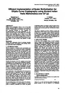
Obviously the latter matrices are sparse but since they do not possess any special structure up to our knowledge, multiplying them by vectors is more expensive than multiplying Vs and Ws . Multiplying elements in the field F36·97 is required in the Tate pairing computation on the group of F397 -rational points of the elliptic curves Ed : y 2 = x3 − x + d d ∈ {−1, 1} defined over F3 . An efficient algorithm for the computation of the Tate pairings on these curves is discussed in [6]. We have implemented the multiplication over F36·97 using the Karatsuba method, the Montgomery method from [18], and our proposed method on a PC with an AMD Athlon 64 processor 3500+. The processor was running at 2.20 GHz and we have used the NTL library (see [19]) for multiplication in F397 . Please note that although we have chosen m = 97 for benchmarking purposes, these methods can be applied to any odd m > 2 as mentioned in Section 3.

Multiplication method Elapsed time (ms) Karatsuba method 1.698 Montgomery method 1.605 Proposed method 1.451 Table 1. Comparison of the execution times of the Karatsuba and Montgomery multipliers with the proposed method for F36m .

The execution times are shown in Table 1. For the Karatsuba and the proposed methods we have used the tower of extensions F397 ⊂ F32·97 ⊂ F36·97 ,

8

where F397 ∼ = F3 [x]/(x97 + x16 + 2) ∼ F397 [y]/(y 2 + 1) F32·97 = F36·97 ∼ = F32·97 [z]/(z 3 − z − 1), whereas for the Montgomery method the representation F36·97 ∼ = F397 [y]/(y 6 + y − 1) has been used. Our implementations show that the new method is almost 14% faster than the Karatsuba and 10% faster than the Montgomery method, which is almost the ratio of saved multiplications. This provides further evidence for the fact that the number of multiplications in F397 is a good indicator of the performance of the method for F36·97 . Our multiplications are based on the following formulas. Let α, β ∈ F36·m be given as: α = a0 + a1 s + a2 r + a3 rs + a4 r2 + a5 r2 s, β = b0 + b1 s + b2 r + b3 rs + b4 r2 + b5 r2 s, where a0 , · · · , b5 ∈ F3m and s ∈ F32·m , r ∈ F6·m are roots of y 2 + 1 and z 3 − z − 1, 3 respectively. Let their product γ = αβ ∈ F36·m be γ = c0 + c1 s + c2 r + c3 rs + c4 r2 + c5 r2 s. The coefficients ci , for 0 ≤ i ≤ 5 are computed using: P0 = (a0 + a2 + a4 )(b0 + b2 + b4 ) P1 = (a0 + a1 + a2 + a3 + a4 + a5 )(b0 + b1 + b2 + b3 + b4 + b5 ) P2 = (a1 + a3 + a5 )(b1 + b3 + b5 ) P3 = (a0 − a3 − a4 )(b0 − b3 − b4 ) P4 = (a0 + a1 + a2 − a3 − a4 − a5 )(b0 + b1 + b2 − b3 − b4 − b5 ) P5 = (a1 + a2 − a5 )(b1 + b2 − b5 ) P6 = (a0 − a2 + a4 )(b0 − b2 + b4 ) P7 = (a0 + a1 − a2 − a3 + a4 + a5 )(b0 + b1 − b2 − b3 + b4 + b5 ) P8 = (a1 − a3 + a5 )(b1 − b3 + b5 ) P9 = (a0 − a3 − a4 )(b0 + b3 − b4 ) P10 = (a0 + a1 − a2 + a3 − a4 − a5 )(b0 + b1 − b2 + b3 − b4 − b5 ) P11 = (a1 − a2 − a5 )(b1 − b2 − b5 ) P12 = a4 b4 P13 = (a4 + a5 )(b4 + b5 ) P14 = a5 b5 c0 = −P0 + P2 − P3 − P4 + P10 + P11 − P12 + P14 ; c1 = P0 − P1 + P2 + P4 + P5 + P9 + P10 + P12 − P13 + P14 c2 = −P0 + P2 + P6 − P8 + P12 − P14 c3 = P0 − P1 + P2 − P6 + P7 − P8 − P12 + P13 − P14 c4 = P0 − P2 − P3 + P5 + P6 − P8 − P9 + P11 + P12 − P14 c5 = −P0 + P1 − P2 + P3 − P4 + P5 − P6 + P7 − P8 + P9 − P10 + P11 − P12 + P13 − P14

9

5

Other applications of the proposed method

Consider the family of hyperelliptic curves Cd : y 2 = xp − x + d d ∈ {−1, 1}

(11)

defined over Fp , for p = 3 mod. 4. Let m be such that (2p, m) = 1 (in practice m will often be prime), and consider the Fpm -rational points of the Jacobian of Cd . An efficient implementation of the Tate pairing on these groups is given by Duursma and Lee in [6] and [20], where they extend analogous results of Barreto et. al. and of Galbraith et. al. for the case p = 3. Notice that this family of curves includes the elliptic curves Ed that we mentioned in the last section. In the aforementioned papers it is also shown that the curve Cd has embedding degree 2p. In order to compute the Tate pairing on this curve, one works with the tower of field extensions Fpm ⊂ Fp2m ⊂ Fp2pm where the fields are represented as Fp2m ∼ = Fp2m [z]/(z p − z + 2d). = Fpm [y]/(y 2 + 1) and Fp2pm ∼ Let a(z), b(z) ∈ Fp2pm [z]≤p−1 , a(z) = a0 + a1 z + . . . + ap−1 z p−1 , b(z) = b0 + b1 z + . . . + bp−1 z p−1 . Then c(z) = a(z)b(z) has 2p − 1 coefficients, two of which can be computed as c0 = a0 b0 and c2(p−1) = a2(p−1) b2(p−1) . In order to determine the remaining 2p − 3 coefficients, we can write a Vandermonde matrix with entries in F∗p2m using, e.g., the elements 1, 2, . . . , p − 1, ±s, . . . , ±

p−3 p−1 s, s. 2 2

Another option is writing a Vandermonde matrix using a primitive 2(p − 1)-st root of unity combined with the relation: c2(p−1) = a2(p−1) b2(p−1) . Notice that there is an element of order 2(p − 1) in Fp2 , since 2(p − 1)|p2 − 1. If a is a primitive element in Fp2 , then ω = a(p+1)/2 is a primitive 2(p − 1)st root of unity.

10

6

Conclusion

In this paper we derived new formulas for multiplication in F36m , which use only 15 multiplications in F3m . Being able to efficiently multiply elements in F36m is a central task for the computation of the Tate pairing on elliptic and hyperelliptic curves. Our method is based on the fast Fourier transform, slightly modified to be adapted to the finite fields that we work on. Our software experiments show that this method is at least 10% faster than other proposed methods in the literature. We have also discussed use of these ideas in conjunction with the general methods of Duursma-Lee for Tate pairing computations on elliptic and hyperelliptic curves.

Acknowledgement The research described in this paper was funded in part by the Swiss National Science Foundation, registered there under grant number 107887, and by the German Research Foundation (Deutsche Forschungsgemeinschaft DFG) under project RU 477/8. We thank also the reviewers for their precise comments.

References 1. Knuth, D.E.: The Art of Computer Programming, vol. 2, Seminumerical Algorithms. 3rd edn. Addison-Wesley, Reading MA (1998) First edition 1969. 2. von zur Gathen, J., Gerhard, J.: Modern Computer Algebra. Second edn. Cambridge University Press, Cambridge, UK (2003) First edition 1999. 3. U.S. Department of Commerce / National Institute of Standards and Technology: Digital Signature Standard (DSS). (2000) Federal Information Processings Standards Publication 186-2. 4. Bailey, D.V., Paar, C.: Optimal extension fields for fast arithmetic in publickey algorithms. In Krawczyk, H., ed.: Advances in Cryptology: Proceedings of CRYPTO ’98, Santa Barbara CA. Number 1462 in Lecture Notes in Computer Science, Springer-Verlag (1998) 472–485 5. Avanzi, R.M., Mih˘ ailescu, P.: Generic efficient arithmetic algorithms for PAFFs (processor adequate finite fields) and related algebraic structures (extended abstract). In: Selected Areas in Cryptography (SAC 2003), Springer-Verlag (2003) 320–334 6. Duursma, I., Lee, H.: (Tate-pairing implementations for tripartite key agreement) 7. Kerins, T., Marnane, W.P., Popovici, E.M., Barreto, P.S.L.M.: Efficient hardware for the tate pairing calculation in characteristic three. In: Cryptographic Hardware and Embedded Systems, CHES2005. Number 3659 in Lecture Notes in Computer Science, Springer-Verlag (2005) 412–426 8. Karatsuba, A., Ofman, Y.: Multiplication of multidigit numbers on automata. Soviet Physics–Doklady 7 (1963) 595–596 translated from Doklady Akademii Nauk SSSR, Vol. 145, No. 2, pp. 293–294, July, 1962. 9. Paar, C.: Efficient VLSI Architectures for Bit-Parallel Computation in Galois Fields. PhD thesis, Institute for Experimental Mathematics, University of Essen, Essen, Germany (1994)

11 10. Lempel, A., Winograd, S.: A new approach to error-correcting codes. IEEE Transactions on Information Theory IT-23 (1977) 503–508 11. Winograd, S.: Arithmetic Complexity of computations. Volume 33. SIAM, Philadelphia (1980) 12. B¨ urgisser, P., Clausen, M., Shokrollahi, M.A.: Algebraic Complexity Theory. Number 315 in Grundlehren der mathematischen Wissenschaften. Springer-Verlag (1997) 13. Bajard, J.C., Imbert, L., Negre, C.: Arithmetic operations in finite fields of medium prime characteristic using the lagrange representation. IEEE Transactions on Computers 55 (2006) 1167–1177 14. Blahut, R.E.: Fast Algorithms for Digital Signal Processing. Addison-Wesley, Reading MA (1985) 15. Cooley, J.W., Tukey, J.W.: An algorithm for the machine computation of the complex fourier series. Mathematics of Computation 19 (1965) 297–31 16. Loan, C.V.: Computational Frameworks for the Fast Fourier Transform. Society for Industrial and Applied Mathematics (siam), Philadelphia (1992) 17. von zur Gathen, J., Shokrollahi, J.: Efficient FPGA-based Karatsuba multipliers for polynomials over F2 . In Preneel, B., Tavares, S., eds.: Selected Areas in Cryptography (SAC 2005). Number 3897 in Lecture Notes in Computer Science, Kingston, ON, Canada, Springer-Verlag (2005) 359–369 18. Montgomery, P.L.: Five, Six, and seven-Term Karatsuba-Like Formulae. IEEE Transactions on Computers 54 (2005) 362–369 19. Shoup, V.: (NTL: A library for doing number theory, http://www.shoup.net/ntl) 20. Duursma, I., Lee, H.S.: Tate pairing implementation for hyperelliptic curves y 2 = xp −x+d. In: Advances in cryptology—ASIACRYPT 2003. Volume 2894 of Lecture Notes in Comput. Sci. Springer, Berlin (2003) 111–123