The upside of such an explicit MPC solution stems from the fact that optimal control input can be obtained on-line by a mere function evaluation. This task can.
Explicit Stochastic MPC Approach to Building Temperature Control J´an Drgoˇna, Michal Kvasnica, Martin Klauˇco and Miroslav Fikar
Abstract— In this paper we show how to synthesize explicit representations of Model Predictive Control (MPC) feedback laws that maintain temperatures in a building within of a comfortable range while taking into account random evolution of external disturbances. The upside of such an explicit MPC solution stems from the fact that optimal control input can be obtained on-line by a mere function evaluation. This task can be accomplished quickly even on cheap hardware. To account for random disturbances, our formulation assumes probabilistic version of thermal comfort constraints. We illustrate how a finite-sampling approach can be used to convert probabilistic bounds into deterministic constraints. To reduce complexity, and to allow for synthesis of explicit feedbacks in reasonable time, we furthermore propose to prune the set of samples depending on activity of constraints. Performance of the stochastic explicit MPC controller is then compared against best-case and worst-case scenarios.
I. I NTRODUCTION Nowadays, energy consumed for heating, cooling ventilation and air conditioning (HVAC) in residential and commercial buildings accounts for roughly 40 % of global energy use [14]. In Europe, this figure is reported to be as high as 76 %. Any reduction of energy demand thus has a huge effect, which goes hand-to-hand with reduction of greenhouse gases and overall level of pollution. It is well known that employing sophisticated control algorithms can decrease energy consumption of HVAC systems in buildings without resorting to modifications of the buildings’ physical construction. Various advanced control methods are nowadays available to achieve this goal, ranging from use of classical PI and state-feedback controllers [6], through methods based on fuzzy systems and neural networks, up to application of optimization-based schemes [17]. Advantage of the latter class is that the task of minimizing energy while respecting thermal comfort can be rigorously stated as an optimization problem, leading to a best-achievable performance. In this paper we also follow the line of devising optimization-based controllers for control of thermal comfort in buildings. Specifically, we consider the class of Model Predictive Control (MPC) strategies [11] which utilize a mathematical model of the building to predict its future behavior. These predictions then allow optimization to select best control inputs that minimize consumed energy while respecting thermal comfort criteria. In real-life situations, however, buildings are subject to external disturbances, such as exterior temperature, solar radiation, or heat generated All authors are with the Slovak University of Technology in Bratislava, Slovakia. {jan.drgona, michal.kvasnica, martin.klauco, miroslav.fikar}@stuba.sk.
by occupancy. Moreover, these disturbances often evolve in a random fashion. Possible ways around would be to consider worst-case MPC which utilizes (often conservative) bounds on possible changes of the disturbances or employing certainty equivalence MPC [12]. Even though such strategies are able to satisfy constraints for arbitrary disturbance, the price to be paid is increased consumption of energy required for heating and cooling. Moreover based on international standards for building control (e.g. ISO 7730), zone control is being used for satysfying the thermal comfort within given range of reliability. This brings us to face the probabilistic constraints, which can not be modeled by standard deterministic procedures, but on the other hand thanks to the knowledge of the probability distributions of the past disturbances, they can be easily modeled by stochastic approaches. Therefore much attention is devoted to stochastic MPC which incorporate random disturbances into probabilistic constraints. However, most of stochastic MPC approaches for building control reported in the literature lead to complex optimization problems [13], [10]. The downside being that complexity of such an optimization is often prohibitive for implementation on cheap process hardware, such as on Programmable Logic Controllers. Therefore in this paper we aim at achieving a simple implementation of stochastic MPC. This is achieved by precomputing, off-line, the optimal solution to a given optimal control problem for all initial conditions of interest using parametric programming [3]. This gives rise to an explicit representation of the MPC feedback law as a Piecewise Affine (PWA) function that maps initial conditions onto optimal control inputs. The upside is that the on-line implementation of such controllers reduces to a mere function evaluation. This task can be performed efficiently even on cheap hardware. However, parametric programming is only applicable to stochastic MPC problems of small size. In our setup, however, the dimensions are large. In particular, the space of initial parameters is 14-dimensional, hence general-purpose explicit stochastic MPC approaches cannot be readily applied. Therefore we show how to formulate the stochastic control problem such that it can be subsequently solved, and such that the solution is not of prohibitive complexity. First, by exploiting the results of [5], we show how to replace stochastic probability constraints by a finite number of deterministic constraints. Subsequently, exploiting a particular dynamics of the building, we show that the number of deterministic constraints can be reduced substantially as to render parametric programming useful. At the end we arrive at an explicit representation of stochastic MPC that achieves a given probability of thermal comfort while
simultaneously minimizing consumption of heating/cooling energy sources. Performance of the proposed stochastic scheme is then compared versus a best-case scenario (which employs fictitious perfect knowledge of future disturbance), and against a worst-case setup that employs conservative bounds on future evolution of disturbances. II. B UILDING M ODELING AND C ONTROL A. Basic Concepts and Tools Mathematical models of physical plants play a vital roles in many areas, including control synthesis, verification and simulation. They represent a mathematical abstraction that should on one hand be sufficiently precise to accurately capture dynamical behavior of the plant and, on the other hand, sufficiently simple as to render control synthesis easy. A wide range of software modeling tools for buildings is nowadays available. Examples include, but are not limited to, TRNSYS [2] and Energy Plus [7]. They usually consider very complex building models based on nonlinear energy and mass balances. Although such models are very accurate, they are not directly suitable for control synthesis due to high complexity. To deal this issue the middleware softwares such as BCVTB [18], and MLE+ [4] were designed for making communication bridges between Matlab and E+. In this work, we have used the ISE (Indoor temperature Simulink Engineering) tool [16], which is based on linear building models. In general, ISE is a free, MATLAB-based modeling tool for simulating the indoor temperature of a building that consists of a single zone. It uses a linear model of the zone and provides a user-friendly graphical interface to Simulink. Contrary to the complex modeling tools mentioned above, models provided by ISE are directly suitable for control synthesis. An another advantage is that ISE is standalone, i.e., it does not rely on any other external software packages. ISE being based on MATLAB/Simulink allows to easily verify performance of various control strategies just by wrapping any MATLAB-based control algorithm as a Simulink S-function. B. Particular Building Model In this paper we consider a linear model of a one-zone building, obtained from ISE. The model has 4 state variables, denoted as x1 to x4 in the sequel. Here, x1 is the floor temperature, x2 represents the internal facade temperature, x3 is the external facade temperature, and x4 stands for the internal room temperature. All temperatures are expressed in ◦ C. The model considers a single control input u, which represents that amount of heat injected to the zone, expressed in watts. Moreover, the model also features 3 disturbance variables d1 , . . . , d3 . Here, d1 is the external temperature (in ◦ C), d2 is the heat generated inside in the zone due to occupancy (in W), and d3 is the solar radiation which heats the exterior of the building (in W). The model can be compactly represented by a linear statespace model in the continuous-time domain x˙ = Ax + Bu + Ed
(1)
where x = [x1 , . . . , x4 ]T is the state vector, x˙ is the state derivative, d = [d1 , . . . , d3 ]T is the vector of disturbances, and and A ∈ R4×4 , B ∈ R4 , E ∈ R4×3 are the state-update matrices. Following values of A, B, E in (1) were extracted from ISE: 2 3 −0.020 0 0 0.020 −0.020 0.001 0.0207 6 0 A = 10−3 · 4 0 0.001 −0.056 0 5 1.234 2.987 0 −4.548 2 3 2 3 0 0 0 0 0 0 7 6 0 7 6 0 B = 10−3 · 4 , E = 10−3 · 4 . 0 5 0.055 0 0 5 0.003 0.327 0.003 0.001
The heating/cooling input u is restricted by −700 W ≤ u ≤ 1400 W.
(2)
Here, positive values of u represent heating, while a negative u stands for cooling. Instead of considering an analytic model for prediction of disturbances, the ISE tool uses historical data for external temperatures (d1 ) and solar radiations (d3 ), captured over the period of 30 days. For the heat generated by occupancy, the ISE model considers d2 = 500 W during office hours, and d2 = 0 W otherwise. C. Control Objectives and Assumptions In this paper we consider that maintaining thermal comfort is equivalent to satisfaction of the following constraint: r − ǫ ≤ x4 ≤ r + ǫ,
(3)
where x4 is the indoor temperature, r is the center of the zone, and ǫ > 0 denotes width of the temperature comfort zone. In the sequel we aim at synthesizing a control policy that manipulates the control input u in (1) such that the indoor temperature respects the constrain in (3), and simultaneously the consumption of energy for heating/cooling is minimized. We assume that at each time instant t we have knowledge of building’s state vector x(t), as well as current values of disturbances d(t). Future disturbances, however, are unknown. To achieve a tractable formulation of the control problem, we therefore assume that we have at least knowledge of the probability distribution of rate of change of disturbances. Hence we assume that we know the probability distribution δ ∼ N (0, σ(t)) (4) such that the future disturbances at discrete time steps t + Ts , . . . , t + N Ts are given by d(t + kTs ) = d(t) + kδ, k = 1, . . . , N,
(5)
where N denotes the prediction window over which the distribution in (4) is deemed reasonably accurate. Hence our goal will be to synthesize the control policy u(t) = µ(x(t), d(t), σ(t)) which minimizes the total energy and maintains thermal comfort over the prediction window N . Because the control authority is limited by (2), and due to the random nature of disturbances, the hard thermal comfort
constraint (3) needs to be relaxed in a probabilistic sense as follows: Pr(x4 ≥ r − ǫ) ≥ 1 − α,
(6a)
Pr(x4 ≤ r + ǫ) ≥ 1 − α,
(6b)
where 1 − α the denotes probability with which the constraints in (3) have to be satisfied for some α ∈ [0, 1]. III. Z ONE T EMPERATURE C ONTROL VIA S TOCHASTIC MPC MPC is control strategy that uses optimization to calculate optimal control inputs. The optimization problem is composed of two parts. The cost function evaluates fitness of a particular predicted profile of predicted variables with respect to qualitative criteria. The task of the optimization is then to compute the optimal profile of predicted control actions for which the cost function is minimized. The set of admissible decisions to choose from is then represented by the constraints of the optimization problem. MPC is implemented in the closed-loop fashion using the principle of receding horizon control. Here, using measurements of state variables at time t, the optimal sequence of control inputs {u∗ (t), . . . , u∗ (t + N Ts )} is first computed by solving the optimization problem. Only the first element of the sequence, i.e., u∗ (t), is then applied to the plant and the procedure is repeated at time t+Ts (where Ts denotes the sampling time), using values of x(t + Ts ). An MPC optimization problem for maintaining high probability of achieving thermal comfort while minimizing energy consumption can be stated as follows: min
u0 ,...,uN
N X
u2k
(7a)
k=0
s.t. xk+1 = Axk + Buk + E(d0 + kδ), Pr(Cxk ≥ r − ǫ) ≥ 1 − α, Pr(Cxk ≤ r + ǫ) ≥ 1 − α, − 700 ≤ uk ≤ 1400, δ ∼ N (0, σ(t)).
Lemma 3.1 ([5]): Let g(u, δ) : RN × Rnd → R be a function that is convex in u for any δ, and let δ be a random variable as in (4). Assume a probabilistic constraint Pr(g(u, δ) ≤ 0) ≥ 1 − α
for some α ∈ [0, 1]. Let δ (1) , . . . , δ (M ) be M samples of the random variable independently extracted from (4). Then the probabilistic constraint in (8) is satisfied with confidence 1 − β, i.e., Pr(Pr(g(u, δ) ≤ 0) ≥ 1 − α) ≥ 1 − β, if g(u, δ (i) ) ≤ 0, i = 1, . . . , M,
(7e) (7f)
Here, xk , uk and dk denote, respectively, values of states, inputs and disturbances predicted at the k-th step of the prediction horizon N , initialized by current measurements of the states x0 = x(t), current disturbances d0 = d(t) and desired center of the thermal comfort zone r = r(t). The predictions are obtained using a discretized version of the LTI model (1) with C = [ 0 0 0 1 ]. Future disturbances predicted in (7b) employ the random variable δ, that follows the probability distribution (7f) where σ(t) is assumed to be available to the optimization. The term d0 + kδ in (7b) originates directly from (5). Due to the probabilistic constraints (7c)-(7d), problem (7) is hard to solve, in general. In this paper we propose to tackle the probabilistic constraint by employing a finite number of realizations of the random variable δ, as captured by the following two lemmas.
(9)
holds for a sufficiently large M . � Lemma 3.2 ([1]): The number of samples M required in Lemma 3.1 is bounded from below by p 1 + N + ln(1/β ) + 2(N + 1) ln (1/β ) . (10) M≥ α �
By employing Lemma 3.1 we can thus replace the probabilistic constraints in (7c)-(7d) by a finite number M of deterministic constraints, each obtained for one of the realizations δ (i) of the random variable. To see this, notice that for (7c) we can set g(·, δ) := r − ǫ − Cxk , where xk embeds δ via (7b). Clearly, g(·, ·) is a single-valued linear function (hence convex) for each k, therefore Lemma 3.1 is applicable. Similar reasoning holds for (7d). In addition, Lemma 3.2 quantifies the lower bound on the number of such realizations, which grows only moderately with the confidence measure β. Consider the i-th realization of the random variable, i.e., δ (i) , and denote by (i) yk
=C
k
A x0 +
k−1 X
k−j−1
A
j=0
(7b) (7c) (7d)
(8)
“ “ ”” Buj + E d0 + (j + 1)δ (i)
!
(11)
the indoor temperature (represented by the 4-th element of the state vector), predicted at the k-th step of the prediction horizon using the disturbance δ (i) . Note that (11) follows directly by solving for yk = Cxk from (7b). Then the MPC optimization problem (7) can be cast as min
u0 ,...,uN
s.t.
N X
u2k
k=0 (i) yk ≥ (i) yk ≤
(12a) r − ǫ, i = 1, . . . , M,
(12b)
r + ǫ, i = 1, . . . , M,
(12c)
− 700 ≤ uk ≤ 1400, (i)
(12d)
where yk is given per (11). Note that (11) serves as a substitution in (12b)-(12c) and is not considered as an equality constraint. By Lemma 3.1, a feasible solution to (12) implies that the probabilistic constraints in the original formulation (7) will be satisfied with a high confidence 1−β. The initial conditions for problem (12) are the current state measurements x0 = x(t), current value of the disturbance vector d0 = d(t), and the M samples δ (1) , . . . , δ (M ) extracted from the probability distribution (4) for a current
value of the standard deviation σ(t). Most importantly, the optimization (12) is a quadratic program in decision variables u0 , . . . , uN since the objective function is quadratic and we have finitely many linear constraints. Therefore a control policy that provides satisfaction of thermal comfort constraints in (6), respects limits of the control authority in (2), and minimizes the energy consumption, can be achieved as follows: 1) At time t, measure x(t), d(t), r(t) and obtain σ(t). 2) Generate M samples δ (1) , . . . , δ (M ) from (4). 3) Formulate the QP (12) and solve it to obtain u∗0 , . . . , u∗N . 4) Apply u(t) = u∗0 to the system and repeat from the beginning at time t + Ts . Remark 3.3: To prevent infeasibility of (12) during transient (for instance when the zone middle point r is changed), it is worth to soften the hard constraints in (12b)-(12c). This can be done by introducing new variables sk , k = 0, . . . , N , and by replacing (12b)-(12c) by (i)
yk ≥ r − ǫ − sk , i = 1, . . . , M,
(13a)
(i) yk
≤ r + ǫ + sk , i = 1, . . . , M. (13b) PN Then the term k=0 qs s2k must be added to (12a) to penalize violation of constraints, together with extra constraints sk ≥ 0, k = 0, . . . , N . The value of the penalization coefficient qs should be selected high as to discourage MPC from violating the constraints unless absolutely necessary. � IV. E XPLICIT S TOCHASTIC MPC F ORMULATION The objective here is to employ parametric programming to pre-calculate the optimal control inputs in (12) for all admissible values of initial conditions. Hence we aim at constructing, off-line, the explicit representation of the optimizer as a function of the vector of initial conditions. Then, once we need to identify the optimal control action on-line for particular measurements, we can replace optimization by a mere function evaluation. This significantly reduces computational requirements of implementation of MPC. Theorem 4.1 ([3]): Let min{U T HU + ξ T F U | GU ≤ W + Sξ}
R
u∗ (t) = [ 1 0 ··· 0 ] U ∗ (ξ) = F˜i ξ + g˜i , if ξ ∈ Ri ,
R
where Fi ∈ RN ×nx , gi ∈ RN , and Ri ⊆ Rnx are polyhedral regions. � To see the relation between Theorem 4.1 and the QP (12), notice that U = [u0 , . . . , uN ] and ξ = [x(t), d(t), r(t), δ (1) , . . . , δ (M ) ]. Moreover, the matrices H, F , G, W , S of (14) can be obtained by straightforward algebraic manipulations, see e.g. [3]. Parameters of the PWA
(16)
where F˜i , g˜i are obtained from Fi , gi by retaining only the first row of a corresponding matrix. � Even though the explicit representation of the MPC feedback law in (16) provides a simple and fast implementation of MPC on embedded hardware, it suffers from the so-called curse of dimensionality. Simply speaking the number of polyhedral regions Ri grows exponentially with the number of constraints in (14). Therefore, from a practical point of view, explicit MPC solutions as in (15) can only be obtained for reasonably simple QP problem (14). Note that our QP has 2N (M + 1) constraints, N decision variables (u0 , . . . , uN ), and 8 + 3M parameters (4 initial states x(t), 3 initial disturbances d(t), 1 center of the thermal comfort zone r(t) and M samples δ (i) , each of which is a 3 × 1 vector). Since M ≫ N in practice due to (10), the main driving factor of complexity is thus M , the number of realizations of the random variable δ employed in (12). To give the reader a flavor of complexity, consider α = 0.05 (which corresponds to a 95 % probability of satisfying the thermal comfort criterion), N = 10, and β = 1 · 10−7 (which means a 99.9999999 % confidence in Lemma 3.1). Then we have M = 919 by (10), hence the QP in (12) has 18400 constraints and 927 parametric variables. Solving such a QP parametrically according to Theorem 4.1 would lead to an explicit solution defined over billions of regions, which is not practical and defeats the purpose of cheap and fast implementation of MPC on embedded hardware. Fortunately, most of the constraints are redundant and can hence be discarded, allowing a tractable solution. To see this, consider the constraint in (12c), rewritten as C(Axk + Buk + E(d0 + kδ (i) )) ≤ r + ǫ.
(14)
be a convex quadratic program with initial conditions ξ ∈ Rnx and decision variables U ∈ RN . Then the optimizer U ∗ of (14) is a piecewise affine (PWA) function of ξ: F1 ξ + g1 if ξ ∈ R1 , .. ∗ (15) U (ξ) = . F ξ + g if ξ ∈ R , R
function U ∗ (ξ) in (15), i.e., gains Fi , gi and polyhedra Ri , can be obtained by a parametric programming solver implemented in the freely-available MPT toolbox[8]. Remark 4.2: For a closed-loop implementation of MPC, only the first element of U ∗ , i.e., u∗0 , needs to be applied to the plant at each time instant. Therefore the explicit recedinghorizon feedback law is given by
(17)
Since the constraint is linear in all variables, it holds if and only max{C(Axk + Buk + E(d0 + kδ (i) ))} ≤ r + ǫ, i
(18)
which is furthermore equivalent to C(Axk + Buk + Ed0 ) + k max{CEδ (i) } ≤ r + ǫ. (19) i
Similarly, we have that (12b) holds if and only if C(Axk + Buk + Ed0 ) + k min{CEδ (i) } ≥ r − ǫ. i
(20)
Let δ = arg maxδ(i) {CEδ (i) }, δ = arg minδ(i) {CEδ (i) }. (21)
Please note that δ and δ are computed over finite set of δ (i) , therefore no optimization is required to determine it’s values. Then for any sample δ (i) with δ ≺ δ (i) ≺ δ the constraints in (12b)-(12c) are redundant. We conclude that, instead of considering M samples δ (i) in (12), one can equivalently state the problem using only the extremal realizations δ, δ, hence M = 2. Using the same figures as above, this leads to a QP with only 60 constraints and 14 parameters in ξ, for which the explicit representation of the optimizer in (14) can be obtained rather easily. Implementation of stochastic explicit MPC thus requires two steps. The first one is performed completely off-line. Here, the QP (12) is formulated using symbolic initial conditions x0 , d0 , r, δ and δ, all concatenated into the vector ξ. Then the QP is solved parametrically for all values of ξ of interest and the explicit representation of the MPC feedback in (16) is obtained by the MPT toolbox. Finally, parameters of the feedback, i.e., the gains F˜i , g˜i , and polyhedra Ri are stored in the memory of the implementation hardware. The on-line implementation of such an explicit feedback is then performed as follows: At time t, measure x(t), d(t), r(t) and obtain σ(t). Generate M samples δ (1) , . . . , δ (M ) from (4). From the generated samples pick δ and δ by (21). Set ξ = [x(t), d(t), r(t), δ, δ] and identify index of the polyhedron for which ξ ∈ Ri . Denote the index of the “active” region by i∗ . 5) Compute u∗ (t) = F˜i∗ ξ + g˜i∗ , apply it to the system and repeat from the beginning at time t + Ts .
1) 2) 3) 4)
Remark 4.3: Identification of δ and δ in (21) does not require any optimization, as the minima/maxima are taken element-wise from a finite set. � There are various ways how to identify index of the active region in Step 4. The most trivial way is to traverse through the polyhedra sequentially, stopping once ξ ∈ Ri is satisfied. Runtime complexity of such an approach is O(R), where R is the total number of polyhedra. More advanced approaches, such as binary search trees [15], can improve the runtime to O(log2 R) by pre-computing a search structure. The amount of memory required to store the PWA function (16) in the memory is linear in R.
V. S IMULATION STUDY AND C ONCLUSIONS To validate performance of the stochastic explicit MPC strategy derived per Section IV, we have assumed a simulation scenario that covered 9 days of historical data. Historical evolution of disturbances (outdoor temperature, heat generated by occupancy, and solar heat) is shown in Fig. 1. The explicit representation of the stochastic MPC feedback strategy (16) was obtained by formulating (12) in YALMIP [9] and solving the QP parametrically by the MPT toolbox. The feedback law covers following ranges of initial
TABLE I C OMPARISON OF VARIOUS STRATEGIES .
Stochastic MPC Best-case MPC Worst-case MPC
Thermal comfort 97.2 % 100.0 % 100.0 %
Consumed energy 125.7 kWh 125.2 kWh 146.0 kWh
conditions: −10 ◦ C ≤ xi (t) ≤ 35 ◦ C, i = 1, . . . , 4, 15 ◦ C ≤ r(t) ≤ 25 ◦ C, 0 ◦ C ≤ d1 (t) ≤ 24 ◦ C, 0 W ≤ d2 (t) ≤ 500 W, 0 W ≤ d3 (t) ≤ 1200 W. Width of the thermal comfort zone was set constantly to ǫ = 0.5 ◦ C. With the prediction horizon N = 10, sampling time Ts = 890 seconds, α = 0.05, and β = 1 · 10−7 , the explicit MPC feedback (16) was obtained as a PWA function that consisted of 816 polyhedra in the 14-dimensional space of initial conditions. Simulated closed-loop profiles of the indoor temperature and consumed heating/cooling energy are shown in Fig. 2. As can be seen, the stochastic controller allows for seldom violations of the thermal comfort zone while maintaining hard limits of the control authority. Overall, the stochastic controller maintains the indoor temperature within the comfort zone for 97.2 % of samples. Performance of the explicit stochastic MPC scheme was then compared to two alternatives. One is represented by a best-case MPC controller, which assumes perfect knowledge of future disturbances over a given prediction horizon. The other alternative is a worst-case scenario which employs conservative bounds on the rate of change of future disturbances. Hence it guarantees satisfaction of constraints in robust fashion, while only minimizing the energy consumption with respect to the worst possible disturbance. Simulated profiles under the best-case and worst-case policies are shown in Fig. 3 and Fig. 4, respectively. Both controllers always managed to keep the indoor temperature within the thermal comfort zone. Moreover, the best-case scenario provides least energy consumption. The worst-case approach, on the other hand, maintains the temperature further away from the boundary of the comfort zone, which leads to an increased consumption of heating/cooling energy. This is a consequence of using conservative bounds on the rate of change of disturbances in the future. Aggregated results are reported in Table I. It should be pointed out that the best-case scenario, although it performs best, is only of fictitious nature since in practice future disturbances are not know precisely. The stochastic scenario, on the other hand, can be easily employed in practice. Moreover, it provides performance comparable to the best-case approach. ACKNOWLEDGMENT The authors gratefully acknowledge the contribution of the Scientific Grant Agency of the Slovak Republic under
d1 (t) [◦ C]
25 20 15 10 5 0
R EFERENCES
[1] T. Alamo, R. Tempo, and A. Luque. On the sample complexity of randomized approaches to the analysis and design under uncertainty. In American Control Conference (ACC), 2010, pages 4671–4676. IEEE, Time [105 s] 2010. [2] W. Beckman, L. Broman, A. Fiksel, S. Klein, E. Lindberg, M. Schuler, 1000 and J. Thornton. TRNSYS: The most complete solar energy system 500 modeling and simulation software. Renewable energy, 5(1):486–488, 0 1994. 0 1 2 3 4 5 6 7 8 [3] A. Bemporad, M. Morari, V. Dua, and E.N. Pistikopoulos. The Time [105 s] explicit linear quadratic regulator for constrained systems. Automatica, 400 38(1):3–20, January 2002. 200 [4] W. Bernal, M. Behl, T. Nghiem, and R. Mangharam. MLE+: a tool for 0 integrated design and deployment of energy efficient building controls. 0 1 2 3 4 5 6 7 8 In Proceedings of the Fourth ACM Workshop on Embedded Sensing 5 Time [10 s] Systems for Energy-Efficiency in Buildings, pages 123–130. ACM, 2012. [5] M. Campi and S. Garatti. The exact feasibility of randomized solutions Fig. 1. Historical trends of disturbances over 9 days. From top to bottom: of uncertain convex programs. SIAM Journal on Optimization, external temperature d1 , solar radiation d3 , and heat generated by occupancy 19(3):1211–1230, 2008. d2 . [6] C. Canbay, A. Hepbasli, and G. Gokcen. Evaluating performance indices of a shopping centre and implementing HVAC control princi22 1400 ples to minimize energy usage. Energy and Buildings, 36(6):587–598, 21.8 1100 2004. 21.6 21.4 [7] D. Crawley, L. Lawrie, F. Winkelmann, W. Buhl, Y. Huang, C. Ped800 21.2 ersen, R. Strand, R. Liesen, D. Fisher, and M. Witte. EnergyPlus: 500 21 creating a new-generation building energy simulation program. Energy 200 20.8 and Buildings, 33(4):319–331, 2001. −100 20.6 [8] M. Kvasnica, P. Grieder, M. Baotic, and M. Morari. Multi-Parametric 20.4 −400 Toolbox (MPT). In Hybrid Systems: Computation and Control, pages 20.2 −700 448–462, March 2004. 20 0 1 2 3 4 5 6 7 8 0 1 2 3 4 5 6 7 8 [9] J. L¨ofberg. YALMIP : A Toolbox for Modeling and Optimization Time [105 s] Time [105 s] in MATLAB. In Proc. of the CACSD Conference, Taipei, Taiwan, (a) Indoor temperature. Dashed lines (b) Heating/cooling. Dashed lines de2004. Available from http://users.isy.liu.se/johanl/ represent the thermal comfort zone. note limits of control authority in (2). yalmip/. [10] Y. Ma, F. Borrelli, B. Hencey, B. Coffey, S. Bengea, and P. Haves. Fig. 2. Performance of the stochastic MPC controller. Model predictive control for the operation of building cooling systems. Control Systems Technology, IEEE Transactions on, 20(3):796–803, 22 2012. 1400 21.8 [11] J.M. Maciejowski. Predictive Control with Constraints. Prentice Hall, 1100 21.6 2002. 21.4 800 [12] Michael J. Messina, Sezai E. Tuna, and Andrew R. Teel. Discrete-time 21.2 500 21 certainty equivalence output feedback: allowing discontinuous control 200 20.8 laws including those from model predictive control. Automatica, −100 20.6 41(4):617 – 628, 2005. 20.4 −400 [13] F. Oldewurtel, A. Parisio, C.N. Jones, M. Morari, D. Gyalistras, 20.2 −700 M. Gwerder, V. Stauch, B. Lehmann, and K. Wirth. Energy efficient 20 0 1 2 3 4 5 6 7 8 0 1 2 3 4 5 6 7 8 building climate control using stochastic model predictive control and Time [105 s] Time [105 s] weather predictions. In American Control Conference (ACC), 2010, (a) Indoor temperature. (b) Heating/cooling. pages 5100–5105. IEEE, 2010. [14] M. Parry, O. Canziani, J. Palutikof, P. van der Linden, and C. Hanson. Fig. 3. Performance of the best-case MPC controller with complete Climate change 2007: impacts, adaptation and vulnerability. Interknowledge of future disturbances. governmental Panel on Climate Change, 2007. [15] P. Tøndel, T. A. Johansen, and A. Bemporad. Evaluation of Piecewise 22 Affine Control via Binary Search Tree. Automatica, 39(5):945–950, 1400 21.8 May 2003. 1100 21.6 [16] A. van Schijndel. Integrated heat, air and moisture modeling and 21.4 800 simulation in hamlab. In IEA Annex 41 working meeting, Montreal, 21.2 500 May, 2005. 21 200 ˇ [17] J. Sirok´ y, F. Oldewurtel, J. Cigler, and S. Pr´ıvara. Experimental 20.8 −100 20.6 analysis of model predictive control for an energy efficient building 20.4 −400 heating system. Applied Energy, 88(9):3079 – 3087, 2011. 20.2 −700 [18] M. Wetter and P. Haves. A modular building controls virtual test 20 0 1 2 3 4 5 6 7 8 0 1 2 3 4 5 6 7 8 bed for the integration of heterogeneous systems. In Third NaTime [105 s] Time [105 s] tional Conference of IBPSA-USA, Berkeley/California, https://gaia. (a) Indoor temperature. (b) Heating/cooling. lbl. gov/bcvtb, 2008. 2
3
4
5
6
7
8
Control input [W] Control input [W]
Control input [W]
Indoor temperature [◦ C]
Indoor temperature [◦ C]
Indoor temperature [◦ C]
d2 (t) [W]
d3 (t) [W]
1
Fig. 4. Performance of the worst-case MPC controller which assumes conservative bounds on future disturbances.
the grant 1/0095/11. The Authors gratefully acknowledge the contribution of the Slovak Research and Development Agency under the project APVV 0551-11.