Apr 22, 2016 - point) x in the measurement volume V, e.g. a receiving antenna, ... wave polarisation, and the orbital part, orbital angular momentum (OAM),.
E XPLOITATION OF A NGULAR M OMENTUM IN W IRELESS C OMMUNICATIONS Bo Thidé1,2 1 Swedish 2 Acreo
Institute of Space Physics (IRF), Uppsala, Sweden Swedish ICT AB, Stockholm/Kista and Hudiksvall, Sweden W IRELESS @KTH F RIDAY SEMINAR E LECTRUM | S TOCKHOLM /K ISTA | S WEDEN 22nd April, 2016
A challenge
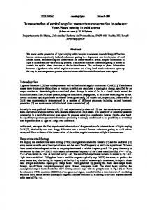
The ‘spectrum crunch’—the increasing congestion of the radio frequency bands—imposes serious limitations on the capacity and capability of existing wireless information infrastructures and on radio science, notably radio astronomy. Are there ways to overcome these limitations already at the fundamental physical level by exploiting underutilised properties of the classical electromagnetic field? We think there are. In order to achieve this, it is necessary to review and rethink the fundamental physical processes that make wireless information transfer possible.
B. Thidé (Uppsala & Stockholm )
Angular Momentum in Wireless Communications
KTH, 2016-04-22
2 / 46
A challenge
The ‘spectrum crunch’—the increasing congestion of the radio frequency bands—imposes serious limitations on the capacity and capability of existing wireless information infrastructures and on radio science, notably radio astronomy. Are there ways to overcome these limitations already at the fundamental physical level by exploiting underutilised properties of the classical electromagnetic field? We think there are. In order to achieve this, it is necessary to review and rethink the fundamental physical processes that make wireless information transfer possible.
B. Thidé (Uppsala & Stockholm )
Angular Momentum in Wireless Communications
KTH, 2016-04-22
2 / 46
Maxwell-Lorentz postulates The microscopic Maxwell equations, formulated by Lorentz, in Dirac’s symmetrised form, allowing for elecric charge density ρ e , magnetic charge density ρ m , electric current density je , and magnetic current density jm ρe ε0 ρm ∇·B = 2 c ε0 ∂B −µ0 jm ∇×E=− ∂t 1 ∂E ∇×B= 2 + µ0 je c ∂t
∇·E =
(1a) (1b) (1c) (1d)
postulate how the electric and magnetic fields E(t, x) ∈ R3 and B(t, x) ∈ R3 , interact, in time t ∈ R and space x ∈ R3 , with the charge densities ρ e,m (t, x) ∈ R and current densities je,m (t, x) ∈ R3 — and vice versa! B. Thidé (Uppsala & Stockholm )
Angular Momentum in Wireless Communications
KTH, 2016-04-22
3 / 46
Fields and observables — two different things! Optics and radio works because it makes use of physical observables. The postulates of classical electrodynamics—Maxwell’s equations—are equations for the fields, which are not directly observable. A quote: “The modern view of the world that emerged from Maxwell’s theory is a world with two layers. The first layer, . . . , consists of fields satisfying simple linear equations. The second layer, . . . , consists of mechanical stresses and energies and forces. The two layers are connected, because the quantities in the second layer are quadratic or bilinear combinations of the quantities in the first layer. To calculate energies or stresses, you take the square of the electric field-strength or multiply one component of the field by another. ··· The unit of energy density is a joule per cubic meter, and therefore we say that the unit of field-strength is the square-root of a joule per cubic meter. This does not mean that an electric field-strength can be measured with the square-root of a calorimeter. It means that electric field-strength is an abstract quantity, incommensurable with any quantitites that we can measure directly.” – Freeman J. Dyson, Why is Maxwell’s Theory so hard to understand? From James Clerk Maxwell Commemorative Booklet, 1999. URL: www.clerkmaxwellfoundation.org/DysonFreemanArticle.pdf “The Nobel committee fleeced him [Dyson] by not awarding his work on quantum electrodynamics with the prize.” – Steven Weinberg B. Thidé (Uppsala & Stockholm )
Angular Momentum in Wireless Communications
KTH, 2016-04-22
4 / 46
Maxwell’s Theory and Quantum Mechanics are related Further, according to Freeman Dyson: “Fields are an abstract concept, far removed from the familiar world of things and forces. ··· The field-equations of Maxwell are partial differential equations. They cannot be expressed in simple words like Newton’s law of motion, force equals mass times acceleration. ··· It may be helpful for the understanding of quantum mechanics to stress the similarities between quantum mechanics and the Maxwell theory. ··· The Maxwell theory became elegant and intelligible only after the attempts to represent electromagnetic fields by means of mechanical models were abandoned. Similarly, quantum mechanics becomes elegant and intelligible only after attempts to describe it in words are abandoned.” – Freeman J. Dyson, Why is Maxwell’s Theory so hard to understand? From James Clerk Maxwell Commemorative Booklet, 1999. URL: www.clerkmaxwellfoundation.org/DysonFreemanArticle.pdf “The Nobel committee fleeced him [Dyson] by not awarding his work on quantum electrodynamics with the prize.” – Steven Weinberg B. Thidé (Uppsala & Stockholm )
Angular Momentum in Wireless Communications
KTH, 2016-04-22
5 / 46
Fields and observables—two different things (2) Things to keep in mind: To allow comparison with experiments, physical processes should be described in quantities that are directly observable and measurable. The fields E and B are not. To study the physics of a classical electromechanical system (charges, currents and fields E and B) only in the fields themselves, or quantities that are linear in these fields, is difficult and problematic. Oftentimes even impossible. The physical observables exploited in radio science and technology are quadratic or bilinear (second-order) in the fields E and B and are conserved quantities (constants of motion).
B. Thidé (Uppsala & Stockholm )
Angular Momentum in Wireless Communications
KTH, 2016-04-22
6 / 46
EM degrees of freedom — the 10 Poincaré invariants The volumetric densities of the 10 Poincaré observables carried by EM fields E(t, x) and B(t, x) are second order (quadratic, bilinear) in these fields. All densities are locally conserved and exhibit an asymptotic |x|−2 ≡ r−2 fall-off: The single scalar quantity field kinetic energy density ε0 (E · E + c2 B · B)/2. Used e.g. in on-off signalling and radiometry (very early radio and optical fibres, cosmic microwave background). The three vector components of the field linear (translational) momentum density ε0 E × B (Poynting vector). Describes changes in the 1D translational EM degrees of freedom. The only conserved EM quantity used fully in today’s radio science, radar and wireless communications. The three pseudovector components of the field angular (rotational) momentum density ε0 (x − xm ) × (E × B). Describes changes in the rotational EM degrees of freedom around a point xm . Used in e.g. photonics, spintronics and orbitronics. Not utilised fully in today’s radio. The three vector components of the field centre of energy. This observable is not utilised at all in today’s optics or radio science or technology. B. Thidé (Uppsala & Stockholm )
Angular Momentum in Wireless Communications
KTH, 2016-04-22
7 / 46
OAM allows a very efficient frequency re-use
α ∆ω+ ∆αm1 +
ω−
ω+
∆αm2 − ∆ω−
B. Thidé (Uppsala & Stockholm )
Horizontal axis: Temporal phase oscillation rate (angular frequency) ω. Vertical axis: Angular phase oscillation rate (OAM) α. Right-hand plane: Right-hand polarisation (SAM σ = +1). Left-hand plane: Left-hand polarisation (SAM σ = −1). All possible squares in the (ω± , α) plane constitute unique, independent information transfer eigenmode channels (ω, σ , αm ). The red and the green squares represent a case when the same identical frequency ω+ = ω− is being re-used six times over.
Angular Momentum in Wireless Communications
KTH, 2016-04-22
8 / 46
Maxwell-Lorentz postulates in Majorana formalism (1) Using the complex-field six-vector (Riemann-Silberstein bivector) G(t, x) = E(t, x) + icB(t, x) and E, B ∈ R3 , and inroducing the complex quantities i i ρ(t, x) = ρ e (t, x) + ρ m (t, x) , j(t, x) = je (t, x) + jm (t, x) c c the Maxwell-Lorentz equations become ρ ∇·G = ε0 i ∂G ∇×G= + icµ0 j c ∂t In regions where ρ = 0 and j = 0 these equations reduce to
where G ∈
C3
∇·G = 0 i ∂G ∇×G= c ∂t B. Thidé (Uppsala & Stockholm )
Angular Momentum in Wireless Communications
KTH, 2016-04-22
9 / 46
Maxwell-Lorentz postulates in Majorana formalism (2) ∇, i.e. setting ∇ = iˆp /}, Using the quantal linear momentum operator pˆ = −i}∇ the Maxwell-Lorentz equations for ρ = 0 and j = 0 take the form pˆ · G = 0 ∂G i} = ciˆp × G ∂t The first equation is the transversality condition p = }k ⊥ G. The second describes the field dynamics. Using the spin-1 angular momentum matrix vector 0 0 0 0 0 i 0 −i 0 S = 0 0 −i xˆ 1 + 0 0 0 xˆ 2 + i 0 0 xˆ 3 0 i 0 −i 0 0 0 0 0 ∇× ) operator, this equation can be written as representation of the curl (∇ i} B. Thidé (Uppsala & Stockholm )
∂G S · pˆ )G = c(S ∂t
Angular Momentum in Wireless Communications
KTH, 2016-04-22
10 / 46
Maxwell-Lorentz postulates in Majorana formalism (3) By introducing the Hamiltonian-like operator ˆ = cS S · pˆ = −ic}S S · ∇ = c|ˆp field |Λˆ H
(5)
S · pˆ field ∑3 Si pˆ field Λˆ = field ≡ i=1 field i |ˆp | |ˆp |
(6)
where
is the helicity operator, we can write the Maxwell-Lorentz curl equation as i}
∂G ˆ = HG ∂t
(7)
i.e. as a Schrödinger/Pauli/Dirac-like equation. This is the well-known Majorana-Oppenheimer representation of the Maxwell-Lorentz postulates (Oppenheimer, 1931; Mignani et el., 1974). We see that G, and hence the fields E and B, can be considered to be of a quantum wavefunction-like character and are therefore ‘incommensurable with any quantitites that we can measure directly’ (Dyson, 1999; Dyson, private communication 2016). B. Thidé (Uppsala & Stockholm )
Angular Momentum in Wireless Communications
KTH, 2016-04-22
11 / 46
EM observables are non-local (averages) dG(t, x, x0) d3x x
x − x0 x − x00
x0
kˆ 0(x, x0) nˆ 0(x)
d3x0 x0 − x00
x0
x00
V0
V
O Figure 1: The electric and/or magnetic charges and currents located in the “physically infinitesimally small” (Rosenfeld, 1965) volume element d3x0 around the point x0 in the source volume V 0 , e.g. a transmitting antenna, with its fixed reference point x00 , give rise to elemental fields in the volume element d3x around the observation point (field point) x in the measurement volume V , e.g. a receiving antenna, with its fixed reference point& Stockholm x0 . ) B. Thidé (Uppsala Angular Momentum in Wireless Communications KTH, 2016-04-22 12 / 46
Maximum exploitation of electromechanical systems Euler showed in 1775 that a complete description and understanding of the dynamics of a physical system requires that one takes both the translational and rotational dynamics of the system properly into account simultaneously. One cannot derive one from the other or vice versa! Translational dynamics is governed by the linear momentum, i.e. force action (Euler’s first law, i.e. a generalisation of Newton’s second law to an arbitrary system of particles). Most existing radio science and information transfer implementations (radio astronomy, radio communications, optics, radar . . . ) are based on the transfer and manipulation of the linear momentum density (Poynting vector). Rotational dynamics is governed by the angular momentum, i.e. torque action (Euler’s second law). The angular momentum has two parts, the spin part, spin angular momentum (SAM), which for EM fields represents wave polarisation, and the orbital part, orbital angular momentum (OAM), representing beam phase twist. Whereas SAM/polarisation has only 2 orthogonal states, σ = ±1, OAM has N = 1, 2, 3, . . . orthogonal states. B. Thidé (Uppsala & Stockholm )
Angular Momentum in Wireless Communications
KTH, 2016-04-22
13 / 46
Conservation of linear (translational) momentum From the Maxwell-Lorentz equations one can derive the global conservation law for the total linear momentum of an electromechanical system dpmech (t) dpfield (t) + + d2x nˆ · T (t, x) = 0 dt dt S where T is the linear momentum flux (Maxwell’s stress tensor), With ρm denoting mass density [kgm−3 ] the mechanical linear momentum is I
pmech (t) =
Z
Z
d3x gmech (t, x) =
V
The EM linear momentum Zis field
p
(t) =
d xg V
d3x ρm vmech
(9a)
d3x ε0 (E × B)
(9b)
V 3
field
Z
(t, x) = V
(8)
Hence, the interpretation of the linear momentum conservation law is Z Z I d d3x ε0 (E × B) + d2x nˆ · T = 0 d3x f + dt V |V{z } | {z } | S {z }
(10)
Force on the matter EM field momentum Linear momentum flow
B. Thidé (Uppsala & Stockholm )
Angular Momentum in Wireless Communications
KTH, 2016-04-22
14 / 46
Electromagnetic linear (translational) momentum (1) The electromagnetic linear momentum carried by the EM field is pfield (t) = ε0
Z
d3x E(t, x) × B(t, x) =
V
1 c2
Z
d3x S(t, x)
V
where S is the Poynting vector. Using B = ∇ × Arotat (vector potential) and applying Helmholtz’s decomposition into rotational (‘transverse’) and irrotational (‘longitudinal’) components, the following exact and manifestly gauge-invariant expression obtains: pfield (t) =
Z V
d3x ρArotat − ε0
B. Thidé (Uppsala & Stockholm )
Z V
∇ × Erotat ) − ε0 d3x Arotat × (∇
Angular Momentum in Wireless Communications
I
⊗ Arotat d2x nˆ · E⊗
S
KTH, 2016-04-22
15 / 46
Electromagnetic linear (translational) momentum (2) In free space, a single temporal Fourier component E(t, x) = E0 (x)e−iωt , for which Erotat = −∂ Arotat /∂t = iωArotat ⇒ Arotat = −iωErotat , carries the cycle averaged classical EM field linear momentum
field � ε0 p = 2}ω
3
∑
Z
i=1 V
∗
d3x (Eirotat ) pˆ Eirotat ,
∇ pˆ = −i}∇
Note the striking similarity with the definiton of the mechanical linear momentum in quantum mechanics, 3 Z
mech � p = ∑ d3x (ψi )∗ pˆ ψi ,
∇ pˆ = −i}∇
i=1 V
where ψi is the ith component of the 3D Schrödinger wave function!
B. Thidé (Uppsala & Stockholm )
Angular Momentum in Wireless Communications
KTH, 2016-04-22
16 / 46
Conservation of angular (rotational) momentum (1) From the Maxwell-Lorentz equations one can readily derive the global conservation law for the total angular momentum of an electromechanical system (e.g. an antenna and the associated EM fields). Integration over the entire volume V , enclosed by the surface S, yields the conservation law for angular momentum with respect to a moment point xm dJmech (t; xm ) dJfield (t; xm ) + + dt dt
I S
d2x nˆ · (x − xm ) × T (t, x) = 0 {z } |
(11)
K (t,x;xm )
The mechanical and electromagnetic angular momentum pseudovectors are Jmech (t; xm ) =
Z
Jfield (t; xm ) =
Z
V V
d3x hmech (t, x; xm ) d3x hfield (t, x; xm ) =
Z
= ε0 B. Thidé (Uppsala & Stockholm )
V
(12a) Z V
d3x (x − xm ) × gfield (t, x) (12b)
3
d x (x − xm ) × (E × B) Angular Momentum in Wireless Communications
KTH, 2016-04-22
17 / 46
Conservation of angular (rotational) momentum (2) We can formulate—and interpret—this global conservation law for the total electromagnetic angular momentum in the following way: d d x (x − xm ) × f + ε0 dt |V {z } | Z
3
Torque on the matter
Z
d3x (x − xm ) × (E × B) V {z } Field angular momentum
(13)
I
+
d2x nˆ · K (t, x; xm ) = 0 |S {z } Angular momentum flow
This angular momentum theorem is the angular analogue of the linear momentum theorem. It shows that the electromagnetic field, as any physical field, carries angular momentum, also known as rotational momentum.
B. Thidé (Uppsala & Stockholm )
Angular Momentum in Wireless Communications
KTH, 2016-04-22
18 / 46
Properties of angular (rotational) momentum (1) The angular (rotational) momentum pseudovector Jfield (t; xm ) = ε0
Z V
d3x (x − xm ) × [E(t, x) × B(t, x)]
can be written as the sum of an intrinsic (independent of choice of moment point xm ) and an extrinsic (dependent of choice of moment point xm ) component, given by the exact and manifestly gauge-invariant expressions field
Σ field
L
Z
(t) = ε0
d3x E(t, x) × Arotat (t, x)
Z V
(t, xm ) =
V
d3x (x − xm ) × ρ(t, x)Arotat (t, x) Z
+ ε0 − ε0
IV S
d3x (x − xm ) ×
�
� � ∇ Arotat (t, x) · E(t, x)
� � d2x nˆ · E(t, x) (x − xm ) × Arotat (t, x)
respectively. B. Thidé (Uppsala & Stockholm )
Angular Momentum in Wireless Communications
KTH, 2016-04-22
19 / 46
Properties of angular (rotational) momentum (2) For a single temporal Fourier component in free space, the cycle averaged classical EM field angular momentum is E
field � D � J (xm ) = Σ field + Lfield (xm ) where D E ε Σfield = 0 2}ω
field � ε0 L (0) = 2}ω
3
∑
Z
j,k=1 V 3
∑
Z
i=1 V
b jk Ek , Σ b jk = −i}εi jk xˆ i = −}S S d3x E ∗j Σ
d3x Ei∗ Lˆ Ei , Lˆ = −i}x × ∇ = −i}εi jk x j ∂k xˆ i
D E b is the spin-1 operator and Σ field is the cycle averaged classical EM Σ field spin angular momentum, SAM, also known as wave polarisation.
� Lˆ is the orbital angular momentum operator and Lfield (0) is the cycle averaged classical EM field orbital angular momentum around xm = 0. B. Thidé (Uppsala & Stockholm )
Angular Momentum in Wireless Communications
KTH, 2016-04-22
20 / 46
EM linear and angular momentum densities for a single Hertzian dipole d = d cos(ωt)ˆz along the polar (z) axis z
z
d
x
d
y
x
y
Figure 2: Angular distribution of the radial Figure 3: Angular distribution of the part of the linear momentum density angular momentum density hfield = hfield ϕˆ , field (Poynting vector) gr . Also known as everywhere directed perpendicular to the zˆ “the radiation pattern.” Minima along the and ϑˆ unit vectors. Minima along the dipole axis and maximum in the equator dipole axis and in the equator plane. B. Thidé (Uppsala & Stockholm ) Angular Momentum in Wireless Communications KTH, 2016-04-22 21 / 46 plane.
EM linear and angular momentum densities for two crossed Hertzian dipoles fed in quadrature z
x
z
y
x
y
Figure 4: Angular distribution of the radial Figure 5: Angular distribution of the z part of the linear momentum density component of the angular momentum (Poynting vector) gfield density hfield r . z . B.T. et al., arXiv:1410.4268 [physics.optics] (2014) B. Thidé (Uppsala & Stockholm )
Angular Momentum in Wireless Communications
KTH, 2016-04-22
22 / 46
The basic idea (1) Consider a beam where the individual electric field vectors E(t, x) expressed in cylindrical coordinates (ρ, ϕ, z) are E(t, x) = E(t, ρ, ϕ, z) = R(ρ)Φ(ϕ)Z(z)T (t)E0
(14)
where E0 = E0 eˆ , E0 being a constant and eˆ a (possibly complex) unit vector, e.g., a linear combination of the two helicity base (bi)vectors. Here Z(z) = Z0 (Ωz)eikz z
(15)
where Z0 (Ωz) is a slowly varying function along the beam (z) axis and kz is the z (longitudinal) component of the wave vector, corresponding to the linear momentum component pz = }kz of each photon of the beam, T (Ωt) = T0 (Ωt)e−iωt
(16)
where T0 (Ωt) is a slowly varying function of time t and ω = kc is the angular frequency, corresponding to the energy }ω carried by each photon of the beam, and R(ρ) is the radial part. B. Thidé (Uppsala & Stockholm )
Angular Momentum in Wireless Communications
KTH, 2016-04-22
23 / 46
The basic idea (2) If the azimuthal part Φ(ϕ) is well-behaved enough, it can be represented by a Fourier series ∞
Φ(ϕ) =
∑
cm eimϕ
(17)
m=−∞
where cm are constants (Fourier amplitudes). Then, the z component of the orbital angular momentum (OAM) is hLfield · zˆ i = hLzfield i = hE(t, x)| Lˆ field |E(t, x)i z
(18)
where ∂ E(t, x) Lˆ field z E(t, x) = −i} ∂ϕ = R(ρ)Z(Ωz)eikz z T (Ωt)e−iωt
∞
∑
cm m}eimϕ E0 (19)
m=−∞ B. Thidé (Uppsala & Stockholm )
Angular Momentum in Wireless Communications
KTH, 2016-04-22
24 / 46
The basic idea (3) This means that the OAM is a weighted superposition of orbital angular momentum (OAM) z component eigenmodes Em (t, x) = E0 R(ρ)Z0 (Ωz)T0 (Ωt)ei(kz z+mϕ−ωt) eˆ
(20)
each exhibiting a helical phase front due to the exp (imφ ) phase factor representing a screw dislocation along the z axis, resulting in an annular distribution of the linear momentum denstiy; for m = 0 the phase front is flat. In particular, Lˆ field |mi = m} |mi z
(21)
which means that the z component of the orbital angular momentum (OAM) of each photon in this beam and therefore of the beam itself is m}.
B. Thidé (Uppsala & Stockholm )
Angular Momentum in Wireless Communications
KTH, 2016-04-22
25 / 46
The basic idea (4) The single-valuedness of the electromagnetic fields upon their winding an integer number of 2π in azimuth angle ϕ around the beam axis z, is manifested in the quantization of the orbital part of the classical electromagnetic angular momentum, resulting in a Bohr-Sommerfeld type quantisation condition (at the classical level!). Mathematically this quantisation can be expressed in terms of Hilbert space orthogonality between the OAM eigenstates |m1 i and |m2 i as follows: hm1 | m2 i =
Z V
d3x Em1 2
�∗
· Em2 2
= |E0 | |T0 (Ωt)|
Z ρ2
2
|R(ρ)| dρ
0
ρ1
×
Z 2π 0
Z z0
eim1
� ϕ ∗
|Z0 (Ωz)|2 dz
eim2 ϕ dϕ = Const × δm1 m2
(22)
where δm1 m2 is the Kronecker delta. B. Thidé (Uppsala & Stockholm )
Angular Momentum in Wireless Communications
KTH, 2016-04-22
26 / 46
OAM can have any non-integer value In the particular case that Φ(ϕ) = eikϕ ρϕ ≡ eiαϕ
(23)
where kϕ is the ϕ (azimuthal) component of the wave vector, and α has a non-integer value, the mth Fourier amplitude in (17) is cm =
exp(iπα) sin(πα) π(α − m)
(24)
Hence, a beam carrying an arbitrary amount α of OAM is a superposition of discrete classical OAM eigenmodes that are mutually orthogonal in a function space sense and therefore propagate independently of each other. An arbitrary angular momentum α therefore exhibits a discrete Fourier spectrum where each angular momentum eigenmode component occupies a bin αm ∈ {α ∈ R; m − 1/2 ≤ α < m + 1/2}, m = 0, ±1, ±2, . . . B. Thidé (Uppsala & Stockholm )
Angular Momentum in Wireless Communications
KTH, 2016-04-22
(25) 27 / 46
The field linear momentum density gfield (t, x) [Poynting vector S(t, x)] vs. the field angular momentum density hfield (t, x; xm ) around an arbitrary moment point xm Property Definition (field point of view)
B. Thidé (Uppsala & Stockholm )
Linear momentum density gfield
= ε0
E × B = S/c2
Angular momentum density hfield (x
Angular Momentum in Wireless Communications
m ) = (x − xm ) × (ε0 E × B)
KTH, 2016-04-22
28 / 46
The field linear momentum density gfield (t, x) [Poynting vector S(t, x)] vs. the field angular momentum density hfield (t, x; xm ) around an arbitrary moment point xm Property Definition (field point of view) SI unit
B. Thidé (Uppsala & Stockholm )
Linear momentum density gfield
= ε0
E × B = S/c2
N m−3 s (kg m−2 s−1 )
Angular momentum density hfield (x
m ) = (x − xm ) × (ε0 E × B)
N m−2 s rad−1 (kg m−1 s−1 rad−1 )
Angular Momentum in Wireless Communications
KTH, 2016-04-22
28 / 46
The field linear momentum density gfield (t, x) [Poynting vector S(t, x)] vs. the field angular momentum density hfield (t, x; xm ) around an arbitrary moment point xm Property Definition (field point of view) SI unit Local conservation law
B. Thidé (Uppsala & Stockholm )
Linear momentum density gfield
= ε0
E × B = S/c2
N m−3 s (kg m−2 s−1 ) ∂ gmech ∂t
Angular momentum density hfield (x
m ) = (x − xm ) × (ε0 E × B)
N m−2 s rad−1 (kg m−1 s−1 rad−1 )
field
+ ∂ g∂t + ∇ · T = 0
Angular Momentum in Wireless Communications
∂ hmech ∂t
field
+ ∂ h∂t
+∇ ·M = 0
KTH, 2016-04-22
28 / 46
The field linear momentum density gfield (t, x) [Poynting vector S(t, x)] vs. the field angular momentum density hfield (t, x; xm ) around an arbitrary moment point xm Property Definition (field point of view) SI unit Local conservation law Fall-off at large distances r
B. Thidé (Uppsala & Stockholm )
Linear momentum density gfield
= ε0
E × B = S/c2
N m−3 s (kg m−2 s−1 ) ∂ gmech ∂t
Angular momentum density hfield (x
m ) = (x − xm ) × (ε0 E × B)
N m−2 s rad−1 (kg m−1 s−1 rad−1 )
field
+ ∂ g∂t + ∇ · T = 0
∼ r−2 + O(r−3 )
Angular Momentum in Wireless Communications
∂ hmech ∂t
field
+ ∂ h∂t
+∇ ·M = 0
∼ r−2 + O(r−3 )
KTH, 2016-04-22
28 / 46
The field linear momentum density gfield (t, x) [Poynting vector S(t, x)] vs. the field angular momentum density hfield (t, x; xm ) around an arbitrary moment point xm Property Definition (field point of view) SI unit Local conservation law
Linear momentum density gfield
= ε0
E × B = S/c2
N m−3 s (kg m−2 s−1 ) ∂ gmech ∂t
Angular momentum density hfield (x
m ) = (x − xm ) × (ε0 E × B)
N m−2 s rad−1 (kg m−1 s−1 rad−1 )
field
+ ∂ g∂t + ∇ · T = 0
∂ hmech ∂t
field
+ ∂ h∂t
+∇ ·M = 0
Fall-off at large distances r
∼ r−2 + O(r−3 )
∼ r−2 + O(r−3 )
Typical phase factor
exp [i(kz − ωt)]
exp [i(kz + mϕ − ωt)]
B. Thidé (Uppsala & Stockholm )
Angular Momentum in Wireless Communications
KTH, 2016-04-22
28 / 46
The field linear momentum density gfield (t, x) [Poynting vector S(t, x)] vs. the field angular momentum density hfield (t, x; xm ) around an arbitrary moment point xm Property Definition (field point of view) SI unit Local conservation law Fall-off at large distances r Typical phase factor Quantal operator (z comp)
B. Thidé (Uppsala & Stockholm )
Linear momentum density gfield
= ε0
E × B = S/c2
N m−3 s (kg m−2 s−1 ) ∂ gmech ∂t
Angular momentum density hfield (x
m ) = (x − xm ) × (ε0 E × B)
N m−2 s rad−1 (kg m−1 s−1 rad−1 )
field
+ ∂ g∂t + ∇ · T = 0
∼ r−2 + O(r−3 )
∂ hmech ∂t
field
+ ∂ h∂t
+∇ ·M = 0
∼ r−2 + O(r−3 )
exp [i(kz − ωt)]
exp [i(kz + mϕ − ωt)]
pˆ z = −i} ∂∂z , (pz = }k, k ∈ R)
Lˆ z = −i} ∂∂ϕ , (Lz = }m, m ∈ Z)
Angular Momentum in Wireless Communications
KTH, 2016-04-22
28 / 46
The field linear momentum density gfield (t, x) [Poynting vector S(t, x)] vs. the field angular momentum density hfield (t, x; xm ) around an arbitrary moment point xm Property Definition (field point of view) SI unit Local conservation law Fall-off at large distances r Typical phase factor Quantal operator (z comp) C symmetry (charge conjugation)
B. Thidé (Uppsala & Stockholm )
Linear momentum density gfield
= ε0
E × B = S/c2
N m−3 s (kg m−2 s−1 ) ∂ gmech ∂t
Angular momentum density hfield (x
m ) = (x − xm ) × (ε0 E × B)
N m−2 s rad−1 (kg m−1 s−1 rad−1 )
field
+ ∂ g∂t + ∇ · T = 0
∼ r−2 + O(r−3 )
∂ hmech ∂t
field
+ ∂ h∂t
+∇ ·M = 0
∼ r−2 + O(r−3 )
exp [i(kz − ωt)]
exp [i(kz + mϕ − ωt)]
pˆ z = −i} ∂∂z , (pz = }k, k ∈ R)
Lˆ z = −i} ∂∂ϕ , (Lz = }m, m ∈ Z)
Even
Even
Angular Momentum in Wireless Communications
KTH, 2016-04-22
28 / 46
The field linear momentum density gfield (t, x) [Poynting vector S(t, x)] vs. the field angular momentum density hfield (t, x; xm ) around an arbitrary moment point xm Property Definition (field point of view) SI unit Local conservation law Fall-off at large distances r Typical phase factor Quantal operator (z comp) C symmetry (charge conjugation) P symmetry (parity/spatial inversion)
B. Thidé (Uppsala & Stockholm )
Linear momentum density gfield
= ε0
E × B = S/c2
N m−3 s (kg m−2 s−1 ) ∂ gmech ∂t
Angular momentum density hfield (x
m ) = (x − xm ) × (ε0 E × B)
N m−2 s rad−1 (kg m−1 s−1 rad−1 )
field
+ ∂ g∂t + ∇ · T = 0
∼ r−2 + O(r−3 )
∂ hmech ∂t
field
+ ∂ h∂t
+∇ ·M = 0
∼ r−2 + O(r−3 )
exp [i(kz − ωt)]
exp [i(kz + mϕ − ωt)]
pˆ z = −i} ∂∂z , (pz = }k, k ∈ R)
Lˆ z = −i} ∂∂ϕ , (Lz = }m, m ∈ Z)
Even
Even
Even (polar/ordinary vector)
Odd (axial vector/pseudovector)
Angular Momentum in Wireless Communications
KTH, 2016-04-22
28 / 46
The field linear momentum density gfield (t, x) [Poynting vector S(t, x)] vs. the field angular momentum density hfield (t, x; xm ) around an arbitrary moment point xm Property Definition (field point of view) SI unit Local conservation law Fall-off at large distances r Typical phase factor Quantal operator (z comp) C symmetry (charge conjugation) P symmetry (parity/spatial inversion) T symmetry (time reversal) symmetry
B. Thidé (Uppsala & Stockholm )
Linear momentum density gfield
= ε0
E × B = S/c2
N m−3 s (kg m−2 s−1 ) ∂ gmech ∂t
Angular momentum density hfield (x
m ) = (x − xm ) × (ε0 E × B)
N m−2 s rad−1 (kg m−1 s−1 rad−1 )
field
+ ∂ g∂t + ∇ · T = 0
∼ r−2 + O(r−3 )
∂ hmech ∂t
field
+ ∂ h∂t
+∇ ·M = 0
∼ r−2 + O(r−3 )
exp [i(kz − ωt)]
exp [i(kz + mϕ − ωt)]
pˆ z = −i} ∂∂z , (pz = }k, k ∈ R)
Lˆ z = −i} ∂∂ϕ , (Lz = }m, m ∈ Z)
Even
Even
Even (polar/ordinary vector)
Odd (axial vector/pseudovector)
Odd
Odd
Angular Momentum in Wireless Communications
KTH, 2016-04-22
28 / 46
OAM allows a very efficient frequency re-use
α ∆ω+ ∆αm1 +
ω−
ω+
∆αm2 − ∆ω−
B. Thidé (Uppsala & Stockholm )
Horizontal axis: Temporal phase oscillation rate (angular frequency) ω. Vertical axis: Angular phase oscillation rate (OAM) α. Right-hand plane: Right-hand polarisation (SAM σ = +1). Left-hand plane: Left-hand polarisation (SAM σ = −1). All possible squares in the (ω± , α) plane constitute unique, independent information transfer eigenmode channels (ω, σ , αm ). The red and the green squares represent a case when the same identical frequency ω+ = ω− is being re-used six times over.
Angular Momentum in Wireless Communications
KTH, 2016-04-22
29 / 46
Approximating a single, monolithic 2D OAM antenna with an array of 1D linear momentum antennas (1)
B. T. et al., Phys. Rev. Lett. 99, 087701 (2007) B. Thidé (Uppsala & Stockholm )
Angular Momentum in Wireless Communications
KTH, 2016-04-22
30 / 46
6.4λ
Linear momentum versus angular momentum (Venice)
ϕ
A0
j0
m=1 m=0
Aπ jπ
Analogue FM transmitter
∆α Detector
Digital QPSK transmitter
520λ
B. Thidé (Uppsala & Stockholm )
Angular Momentum in Wireless Communications
KTH, 2016-04-22
31 / 46
Linear momentum versus angular momentum in a reflective environment (1) Mirror
pfield 1
pfield 2
pfield 1
pfield 0 Transmitter
pfield 2
pfield 0
pfield 0 Receiver
Figure 6: Communicating with electromagnetic linear momentum pfield in the presence of a mirror. In the two-dimensional plane of the figure, the vector pfield propagates 0 directly along the straight path to the receiver, while the vector pfield is reflected off the 1 mirror without recoil and produces the vector pfield at the receiver. Since pfield is a 2 constant of the motion and preserves its parity upon reflection the full 3D structure of the EM linear momentum can be obtained by postprocessing. This is used in present MIMO schemes for enhancing the spectral density of linear-momentum radio communications in reflective environments. Cf. Andrews et al., 2001. B. Thidé (Uppsala & Stockholm )
Angular Momentum in Wireless Communications
KTH, 2016-04-22
32 / 46
Linear momentum versus angular momentum in a reflective environment (2) Mirror
Jfield 1
Jfield 2
Jfield 1
Jfield 0 Transmitter
Jfield 2
Jfield 0
Jfield 0 Receiver
Figure 7: Communicating with electromagnetic angular momentum in the presence of a mirror. The electromagnetic angular momentum Jfield is a pseudovector and therefore suffers a parity change when it is reflected off a dense medium. Taking this parity change into account properly, the reflected pseudovector can be used in MIMO-type schemes for enhancing the spectral density of angular-momentum radio communications, over and above the enhancement offered by the multi-state quantal capability of angular momentum itself relative to the single-state linear momentum. B. Thidé (Uppsala & Stockholm )
Angular Momentum in Wireless Communications
KTH, 2016-04-22
33 / 46
Linear momentum versus angular momentum in a reflective environment (3) Simulation 01
11
Quadrature phase
1
0
−1 00
10 −1
0 In phase
1
Figure 8: Numerically simulated constellation diagram for the QPSK information transfer. B. Thidé (Uppsala & Stockholm )
Angular Momentum in Wireless Communications
KTH, 2016-04-22
34 / 46
Linear momentum versus angular momentum in a reflective environment (4) Experiment 01
11
Quadrature phase
1
0
−1 10
00 −1
0 In phase
1
Figure 9: Constellation diagram for the QPSK information transfer as measured in the experiment in the presence of ground reflections and an interfering FM signal at the same carrier frequency. B. Thidé (Uppsala & Stockholm )
Angular Momentum in Wireless Communications
KTH, 2016-04-22
35 / 46
Approximating a single, monolithic 2D OAM antenna with an array of 1D linear momentum antennas (2)
B. T. et al., Phys. Rev. Lett. 99, 087701 (2007) B. Thidé (Uppsala & Stockholm )
Angular Momentum in Wireless Communications
KTH, 2016-04-22
36 / 46
N-tupling the capacity of each polarisation state in a radio link using only EM angular momentum (1)
Three separate OAM antennas (helicoidal parabolic antennas with radomes) ensure that the three overlapping beams are pure OAM Lz eigenstates with azimuthal quantum numbers m = −1, 0, +1, respectively.
Tamburini et al., Radio Sci. 50, 1–8 (2015) B. Thidé (Uppsala & Stockholm )
Angular Momentum in Wireless Communications
KTH, 2016-04-22
37 / 46
N-tupling the capacity of each polarisation state in a radio link using only EM angular momentum (2)
Single-frequency long-range wireless communication with more than two channels per polarisation state is difficult to realise in an efficient way with linear-momentum multiport techniques since those techniques require long antenna baselines and heavy digital signal post-processing. Tamburini et al., Radio Sci. 50, 1–8 (2015) B. Thidé (Uppsala & Stockholm )
Angular Momentum in Wireless Communications
KTH, 2016-04-22
38 / 46
N-tupling the capacity of each polarisation state in a radio link using only EM angular momentum (3) (a) Linear momentum density intensity gfield = |ε0 E × B|. (b) Phase map for the beam in the OAM eigenstate with azimuthal quantum number (topological charge) −1. (c) OAM state spectrum obtained at the receiving end. (d) Numerically simulated phase map. Tamburini et al., Radio Sci. 50, 1–8 (2015) B. Thidé (Uppsala & Stockholm )
Angular Momentum in Wireless Communications
KTH, 2016-04-22
39 / 46
N-tupling the capacity of each polarisation state in a radio link using only EM angular momentum (4)
4QAM constellation diagrams for all three orthogonal OAM eigenstates m = l ∈ {−1, 0, +1} transmitted simultanously between the two end points of one and the same radio link. No polarisation, no MIMO techniques, and no extra frequency bandwidth was used. Tamburini et al., Radio Sci. 50, 1–8 (2015) B. Thidé (Uppsala & Stockholm )
Angular Momentum in Wireless Communications
KTH, 2016-04-22
40 / 46
Angular momentum density hfield (0) = x × (ε0 E × B), along a ring around a turnstile antenna
Figure 10: Angular momentum density hfield (0) along a circular ring in the plane of two crossed dipole antennas located at the origin x = 0 and fed in quadrature. Integration over the ring shows that it experiences a mechanical angular momentum R Jmech (t, 0) = Jfield (t, 0) = ring d3x hfield (t, x, 0) and a torque τ mech = dJmech /dt. B. Thidé (Uppsala & Stockholm )
Angular Momentum in Wireless Communications
KTH, 2016-04-22
41 / 46
Suspension G
Ring
Turnstile Iantenna C A
Acceleration (x10-4 °/s2)
Microwave version of the Einstein-de Haas experiment — Torque on a copper ring subject to EM angular momentum 4
Right
2 Power (W )
0
10
20
30
-2 -4
Left
A
A turnstile antenna radiates angular Acceleration vs. radiated angular momentum momentum at 870 MHz. It transfers power for π/2 dephasing (red) and −π/2 detorque to the conduction electrons in phasing (blue). Full drawn lines: Theoretical a copper ring and hence to the ring model. Crosses: Experiment. itself acting as a torsion pendulum. Emile et al., Phys. Rev. Lett., Vol. 112, p. 053902, 5 Feb 2014 B. Thidé (Uppsala & Stockholm )
Angular Momentum in Wireless Communications
KTH, 2016-04-22
42 / 46
A two-dimensional optomechanical transducer for radio Nano-mechanical oscillators can couple strongly to either microwave or optical fields. When a radio signal hits a voltage biased membrane, a 2D antenna current density distribution, perpendicular to the membrane, will result, thus enabling the detection of OAM. The detection can be made by a laser beam that senses the mechanical motion of the membrane. For a transducer operating at room temperature (300 K), a noise temperature of 1 K has been experimentally demonstrated. A noise temperature of 40 mK and a sensitivity limit of 5 pV/Hz1/2 has been projected. Bagci et al., Optical detection of radio waves through a nanomechanical transducer, Nature, Vol. 507, Issue 7490, pp. 81–85 (2014) B. Thidé (Uppsala & Stockholm )
Angular Momentum in Wireless Communications
KTH, 2016-04-22
43 / 46
EM fields by spin currents (1)
B. Thidé (Uppsala & Stockholm )
Angular Momentum in Wireless Communications
KTH, 2016-04-22
44 / 46
EM fields by spin currents (2)
B. Thidé (Uppsala & Stockholm )
Angular Momentum in Wireless Communications
KTH, 2016-04-22
45 / 46
New possibility: Orbitronics (atomtronics)
B. Thidé (Uppsala & Stockholm )
Angular Momentum in Wireless Communications
KTH, 2016-04-22
46 / 46