Int. J. Sensor Networks, Vol. X, No. Y, XXXX
Exploiting architectural techniques for boosting base-station anonymity in wireless sensor networks Zhong Ren* and Mohamed Younis Department of Computer Science and Electrical Engineering, University of Maryland, Baltimore County, Baltimore, MD, USA Email:
[email protected] Email:
[email protected] *Corresponding author Abstract: Wireless Sensor Networks (WSNs) often serve mission-critical applications in hostile environments and may be thus a subject to attacks. Since the sensor data are collected at in situ base-station (BS), an adversary can inflict the maximal damage to a WSN by pinpointing the BS. In this paper, we propose three novel approaches for boosting the anonymity of the BS nodes to protect them from potential threats. We first explore the deployment of multiple BS nodes and provide guidelines on a cost versus anonymity trade-off to determine the most suitable BS count for a network. Second, we exploit the mobility of BS nodes and categorise the effect of relocating some of the existing BS nodes to the lowest anonymity regions. Finally, we pursue dynamic sensor to cluster re-association in order to change the traffic pattern and confuse the adversary. The effectiveness of the proposed approaches is validated through simulation. Keywords: WSNs; wireless sensor networks; anonymity; traffic analysis; location privacy. Reference to this paper should be made as follows: Ren, Z. and Younis, M. (XXXX) ‘Exploiting architectural techniques for boosting base-station anonymity of wireless sensor networks’, Int. J. Sensor Networks, Vol. X, No. Y, pp.xxx–xxx. Biographical notes: Zhong Ren is a Software Development Engineer at Amazon.com. He attended University of Maryland, Baltimore, from 2009 to 2011 for master degree in Computer Science. He received his bachelor degree in Computer Science from National University of Singapore in 2007. He worked on Tivoli security products at IBM for two years before attending graduate school. His main research focus during the graduate school was security and anonymity, especially in wireless sensor networks. Mohamed F. Younis is currently an Associate Professor in the CSEE department at UMBC. Before joining UMBC, he was with Honeywell International Inc., where he led multiple projects for building integrated fault tolerant avionics and dependable computing infrastructure. His technical interest includes network architectures and protocols, embedded systems, fault tolerant computing, and secure communication. He has published over 160 technical papers in refereed conferences and journals. He has five patents. He serves/served on the editorial board of multiple journals and the organising and technical programme committees of numerous conferences. He is a senior member of the IEEE.
1
Introduction
Wireless Sensor Networks (WSNs) have shown great potential for serving a full spectrum of applications in a wide variety of environments (Akyildiz et al., 2002; Chong and Kumar, 2003). Of special interest are applications that operate in hostile setups such as combat zones and territorial border. These applications are categorised with the presence of adversaries who are eager to attack the network. A WSN is typically composed of a large set of miniaturised sensor nodes that report their findings to a nearby base-station (BS). The BS tasks the sensor nodes, processes the data and interfaces the network to remote users. The important role that the BS plays
Copyright © 200X Inderscience Enterprises Ltd.
makes it a critical asset for the network and would thus become a target of adversary’s attack. The adversary will focus all efforts on uncovering the identity and location of the BS in order to launch attacks to disrupt or damage the BS. In fact, given the unattended network operation, the adversary can even capture the BS and extract stored sensitive information or replace the BS with a malicious one. Therefore, keeping BS’s identity and location anonymous is of utmost importance in WSNs. Since the sensor nodes are battery-operated and have a limited lifespan, multi-hop routes are usually pursued to disseminate the collected data to the BS (Akyildiz et al., 2002). Since the BS serves as the sink of all data traffic, an
Z. Rhen and M. Younis adversary would try to determine the routing topology to identify the BS. Contemporary anonymous routing techniques (Boukerche et al., 2004; Zhang et al., 2005; Seys and Preneel, 2006) cipher the packet header in order to conceal the ID of the BS so that the adversary cannot extract it from an intercepted packet. However, anonymous routing does not suffice since the adversary can still pursue link layer based analysis. Basically, the adversary would intercept RF transmission, localise the source and determine the range. By correlating the intercepted transmissions both spatially and temporally the adversary can detect links between nodes and aggregate that to form data paths. Such traffic analysis can uncover the position of the BS and make the network vulnerable. A number of techniques have been proposed in the literature for boosting the BS’s anonymity. Most of these techniques focus on concealing BS’s role by spreading the network traffic to disguise the role of BS as a sink (Deng et al., 2005; Conner et al., 2006; Acharya and Younis, 2010), preventing hop-to-hop packet tracing (Ebrahimi and Younis, 2011) and relocating the BS (Acharya and Younis, 2010). However, all the techniques have assumed network architectures with a single BS node. No study has been conducted for networks with multiple BS nodes and assessed their impact on anonymity. In addition, although relocating the BS to a safer spot has been pursued, no prior work has exploited the possibility that a mixture of mobile and stationary BS nodes are deployed and tried to take advantage of that in boosting the anonymity. This paper fills this gap and studies the impact of the number and mobility of the BS nodes on anonymity. The goal is to provide guidelines for the network designers in order to determine the appropriate resources and node capabilities and conduct trade-off between anonymity and other metrics like cost. Furthermore, many techniques have been proposed to group sensors into clusters and assign them to one out of the multiple BS that a WSN may have (Abbasi and Younis, 2007). The primary objective of these techniques is to achieve balanced network load among the BS nodes during the network operation. In this paper, we exploit the idea of dynamic sensor to cluster re-association in order to change the traffic pattern within the individual clusters and boost the anonymity of the BS. Each sensor makes on-the-fly decision about which BS it reports to, based on anonymity measurement. All proposed techniques are validated through extensive simulation experiments. The rest of the paper is organised as follows. Section 2 describes the considered system and adversary models. Section 3 summarises related work. Section 4 discusses the goals, metric and our proposed approaches for boosting the BS anonymity. The simulation results are discussed in Section 5. Finally, Section 6 concludes the paper.
2
System model
In this section, we describe the network operation and adversary models that we assume in this paper.
Network model: In this paper, we consider the most typical WSN model. All the sensor nodes have limited but similar capabilities including energy, communication range and link bandwidth. Besides sensor nodes, there will be one or multiple BS in the WSN. The BS nodes are of two types: stationary and mobile. A mobile BS is able to move within the WSN area as needed. The BS serve as data sink of all data traffic originated at the sensors. In the presence of multiple BS, each sensor node picks the closest BS to send the data packets. Figure 1 shows an illustration of an example of the considered WSN model. Figure 1
Notes:
Illustration of a WSN conducting target tracking in a battlefield (see online version for colours)
The radio towers represent a stationary BS, the truck with mounted antenna represents a mobile BS, the tank represents the target of interest, and the small circles represent the homogeneous sensors distributed in the battlefield. Whenever the tank moves into the detection range of nearby sensors (dark circle), the sensors will report its location to one of the BS nodes. Since there are multiple BS nodes in the network, the data packets are forwarded to the closest BS along the least cost path. The hollow circles represents sensor that are not transmitting data, the light circles represent the nodes that forward the data packet to the destination BS node along the path indicated by the arrows.
It is assumed that sensors know their positions relative to the BS nodes by applying localisation algorithm as indicated by Youssef et al. (2005). Least-cost multi-hop routes are pursued for disseminating data packet to the BS with communication energy used as the link cost. In addition, it is assumed that an anonymous routing protocol as mentioned by Seys and Preneel (2006) is employed in order to conceal the identity of the BS nodes while ensuring the data integrity and authenticity of the source of packets. Precautionary measures are assumed to be employed in the design and the operation of the BS in order to avoid exposing it. For example, a BS does not use long-haul transmissions and limits its involvement in control traffic, e.g. new route discovery, in order to keep itself undistinguishable from sensor
Exploiting architectural techniques for boosting base-station anonymity nodes. It is also assumed that camouflage techniques have been applied to the BS so that adversary cannot identify them visually, even if she/he is in the vicinity of BS unless an exhaustive and thorough search is conducted. In addition, mobile BS nodes would move cautiously and covertly so that the adversary cannot detect them. Adversary model: Because the WSNs in hostile environments are likely to be used for sensitive and confidential applications, well-equipped and highly motivated adversary should be expected. We envision an adversary with the aim to physically destroy BS. For the capabilities of the adversary, it is assumed that adversary is equipped with powerful antenna and can intercept and localise all radio communication in the network deployment area. The adversary may use signal-detection techniques such as angle of arrival, received signal strength, etc. (Li et al., 2005; Yang et al., 2007) and then apply localisation algorithms (Savvides et al., 2001; Niculescu and Nath, 2003) in order to determine the position of the individual nodes. The adversary then performs correlation of the intercepted transmissions to identify active communication links and the data paths. To facilitate the traffic analysis, the adversary divides the entire area into a number of equal-sized cells. The size of a cell reflects the accuracy of the localisation of the source of the RF transmission, i.e. the adversary cannot accurately distinguish between the different sensors within a cell. Based on the transmission power, the adversary determines the neighbouring cells that potentially host the recipient. In other words, the traffic analysis is performed on the level of cells with the goal of finding out the cell that has the BS. The adversary is mobile and can move from one physical location to another. In reality the adversary can mount antennas on a vehicle or a robot and hovers around the WSN area. Upon identifying the BS cell, the adversary conducts an exhaustive search and may use careful and thorough visual inspection to recognise the BS. While the adversary can intercept packets, it is assumed that the cryptosystem is so robust that the adversary cannot apply cryptanalysis to decrypt the contents of the packets. The adversary is also assumed to be a passive listener and does inject his own packet into the network.
3
Related work
Because its role as a data collector, uneven network traffic will be created around the BS. Therefore, one of the major issues is how to balance the network traffic throughout the network and also hide the fact that data packets are converging to the BS. The work of Deng et al. (2005), Conner et al. (2006), and Acharya and Younis (2010) strive to address this challenge. Deng et al. (2005) introduced a set of algorithms to defend against traffic analysis. First, they proposed a multi-parent scheme, where each sensor has multiple parents on the routing tree and randomly chooses a parent to forward packets. The second technique is introduced called random walk. In both of these techniques
randomness is introduced in the data forwarding path to the BS. The third technique is called fake path, where redundant packets are injected into the network in order to mislead the adversary into believing that the BS at the destination of the redundant packets. Conner et al. (2006) proposed to use data aggregators to disguise the real location of the BS. Aggregators are called decoy sinks with data packets forwarded to them, and then they process and aggregate the sensor readings before sending to the real BS. The major problem with this approach is that a decoy sink under this assumption is a de facto BS. If adversary takes out the decoy sink, the network operation will be disrupted as well. Acharya and Younis (2010) proposed the BAR approach. The idea is simply to make the BS disguises itself by transmitting BAR packets with varying intensity to its neighbour when it receives data packets. The possibility of re-transmitting BAR packet diminishes each time the BAR packet is forwarded. BAR packets can be forwarded away to a region far away from the BS and mislead the adversary into believing that the BS is just an intermediate forwarding sensor. The BS relocation is also studied by Acharya and Younis (2010). The paper presents guidelines for when, where and how to move the BS. A relocation technique is introduced in order to safeguard BS while moving. Meanwhile, the approach of Youssef and Younis (2010) changes the transmission power of the individual sensors in order to increase the node degree and complicate the traffic analysis and slow its convergence. Although the above mentioned approaches have helped increasing the anonymity of the BS to some extent, they all have made the assumption that there exists only one BS. While multiple BS nodes have been studied extensively under other metrics like data latency and energy conservation (Younis et al., 2006, Youssef and Younis, 2010), no study has exploited the impact of multiple BS nodes on anonymity or tried to use a mixture of mobile and stationary BS nodes to boost BS anonymity. On the other hand, grouping nodes into clusters has been pursued by many researchers as a means for efficient network management. Clustering algorithms in WSNs usually elect a cluster-head (CH) to manage the sensors within the group. Published approaches vary in the way they choose a CH, and in the criteria of assigning sensors to a cluster (Abbasi and Younis, 2007). A CH can be either statically appointed, or elected among the peer sensors, or based on a predefined round robin schedule (Heinzelman et al., 2000; Bandyopadhyay and Coyle, 2003; Younis and Fahmy, 2004; Youssef and Younis, 2010). Different layers of clustering can be utilised to build a hierarchical network (Bandyopadhyay and Coyle, 2003; Younis et al., 2006), multiple attributed and objectives may be factored by Heinzelman et al. (2000), Banerjee and Khuller (2001), Shen and Shi (2008) and Youssef et al. (2009) and the sensors’ membership in a cluster can be fixed or variable (Erciyes et al., 2007). However, these approaches do not consider location privacy issues. In WSNs with multiple BS nodes, it is typical to designate the powerful BS as a CH rather than a sensor. If sensor nodes are not uniformly distributed around the BS nodes the clusters formed will have different load, which will affect the lifetime and energy consumption of the system. Gupta and Younis
Z. Rhen and M. Younis (2003) introduced an approach to cluster unattended wireless sensors while balancing the load among the clusters in order to increase the node lifetime and lower processing delay. However, this approach is static and does not factor any anonymity concern. In this paper, we exploit dynamic association of sensor to clusters so that the traffic pattern changes and the traffic intensity gets equalised in the various clusters and consequently the adversary will have hard time correlating the transmissions and determining the data paths. The approach of Blace et al. (2008) factors in the threats that a node is exposed to in the selection of CHs. However, application-level metric is used in assessing the threats and the potential of traffic analysis is not considered.
4
Boosting base-station anonymity
This section first explains the metric used for assessing the BS anonymity and then describes our proposed approaches for increasing the BS anonymity in WSNs.
4.1 Anonymity evaluation In order to quantify the BS anonymity, we employ the modified version of GSAT test proposed by Acharya and Younis (2010). The GSAT test was first proposed by Deng et al. (2005) as a tool for measuring the average number of steps an adversary makes until finding the cell where the BS is located. The idea is to proceed in a greedy manner by identifying radio transmission/ reception hot spots and gradually move to the area where the BS is stationed. The adversary starts from a random cell and monitors radio communication within its vicinity, which includes its own cell and all the adjacent cells. After a certain period of time, the adversary counts the radio activities that were intercepted and moves to the neighbouring cell with the highest transmission count. If the adversary’s cell experiences the most activities, the search for the BS is said to be stuck at a local maxima. In such a case, the adversary randomly chooses an adjacent cell to move to. The greedy search terminates if the BS cell is reached, and the corresponding number of moves that the adversary takes is said to be the GSAT number. However, given the assumed adversary capabilities, the adversary will not be able to visually identify the BS even if it is in the same cell, the GSAT test will never terminate unless the adversary pauses for long time, every time a local maximum is encountered. In the modified version of GSAT (Acharya and Younis, 2010), the total number of moves taken and the number of times the adversary visits the individual cells are tracked. At any given time t, the GSAT score of a cell i is defined as: No. of cell visits G ( i, t ) = No. of total moves
The GSAT score of all the cells at time t should sum up to 1, i.e.
n
∑ G ( i, t ) = 1 , where n is the total number of cells. i
The GSAT score is a very helpful indicator for whether a cell hosts the BS. Since all data packets must ultimately be forwarded to BS, it is inevitable to have the BS cells as radio
activity hot spots. This uneven traffic pattern especially helps the adversary in assessing the likelihood that a cell hosts the BS. GSAT score captures the essence of WSN traffic pattern: if an adversary visits one particular cell again and again due to its high activities count, it can be concluded with high confidence that the BS resides in that cell. The GSAT-based anonymity assessment is illustrated in Figure 2. In Figure 2 the radio tower presents the BS, the dark circle presents the initial location of the adversary, the dotted circles presents the location of adversary in each steps and the centred number associated with each cell presents the number of radio transmission happened in the cell. As demonstrated, the adversary divides the WSN into 16 cells with the aim to locate BS. It is assumed that adversary can monitor traffic in all adjacent cells. Adversary first starts in Cell 4 while BS is located in Cell 10. In Step 1, adversary monitors network traffic in Cell 3, 4, 7 and 8; among them Cell 8 has the highest radio activities count 201. Therefore, adversary moves to Cell 8. The same is applied in Step 2 and Step 3. After Step 3, BS is stuck in local maxima, where all adjacent cells have radio activity counts lower than its current Cell 10. This is because BS also is located in Cell 10, although the adversary cannot visually notice it. In Step 4, the adversary randomly selects Cell 14 to move to because it is stuck in local maxima after Step 3. In Step 5, because of the high activity count in Cell 10, the adversary moves back again to Cell 10 from Cell 14. In this process the adversary has made five moves in four cells. Since GSAT = no. of cell visit/no. of total visit, after Step 5, Cells 8, 11 and 14 will have GSAT score 1/5 = 0.2. Cell 10 is visited twice, therefore, having GSAT score 2/5 = 0.4. All other cells not visited by adversary have GSAT score 0. Figure 2
An example to illustrate how the GSAT score is calculated (see online version for colours)
If only one BS serves the network, the measurement of anonymity of that BS is very straightforward, namely the GSAT score of the BS cell. However, since in our study, multiple BS will be deployed, each one of them will have their own GSAT scores. Therefore, we will use two aggregate anonymity metrics: the Average GSAT and the Max GSAT of a BS. The Average GSAT represents the Average GSAT scores for the cells that have BS nodes. Max GSAT reflects the maximum GSAT score among all the BS cells, which points out the least protected BS.
Exploiting architectural techniques for boosting base-station anonymity
4.2 Exploiting BS count and mobility The effect of the BS count on the WSN performance has been studied in the literature (see e.g. Younis et al., 2006; Youssef and Younis, 2010). However, the focus has been mostly on contemporary WSN performance metrics such as data delivery delay, node lifetime and network connectivity. The general conclusion of these research efforts is that adding more BS nodes will boost the performance since the traffic will be spread, multiple BS nodes will share the burden of receiving the incoming sensor data reports, and the data paths will be shorter. Since the BS nodes are significantly more expensive than sensors, a performance and cost trade-off exists. In this paper, we propose to deploy multiple BS nodes to boost both the anonymity of BS nodes in terms of both average and Max GSAT. Since the availability of multiple BS nodes reshapes the routing topology and spreads the traffic, fewer and less recognisable traffic hot spots will exist in the vicinity of the individual BS nodes and consequently the anonymity will get positively impacted. The question is whether there is a ceiling on the performance gain and whether there is a certain BS count after which the anonymity is not further enhanced. In Section 5, we quantify the effect of the BS count on anonymity through simulation in order to provide a base for anonymity, performance and cost trade-off that the network designer can exploit. We further propose combining the effect of BS multiplicity and mobility on anonymity. As mentioned in Section 3, relocating the BS has been exploited by Acharya and Younis (2010) as means for nullifying the traffic analysis and forcing the adversary to start from scratch. We opt to assess the performance when the network is served by K mobile BS nodes out of the M base-stations that are deployed. We study the effect of varying K on the anonymity performance. Again, the study will assist the network architect in allocating the required resources since a mobile BS is more expensive and challenging to design than a stationary one. As recommended by Acharya and Younis (2010), a relocated BS will be moved to the cell with the least GSAT score. In the proposed approach, a mobile BS monitors the GSAT scores of all cells, and after a preset time period, it identifies the cell with lowest GSAT score and moves to it. If there are multiple mobile BSs, i.e. K > 1, the K cells with the lowest GSAT score are picked and each mobile BS moves to the closest cell among them. Although the GSAT score is a measurement from the perspective of an adversary, each BS simulates the behaviour of adversaries and keeps track of GSAT scores. With knowledge of its own GSAT and GSAT scores of other cells of WSN, mobile BS can pursue location adjustment in order to reduce its vulnerability to adversary’s attacks. Figure 3 shows a detailed example for the proposed mobile BS relocation in a multi-BS set-up. In Figure 3 the BS nodes are represented by dark circles, and their respective future locations and travel paths are represented by hollow circles and arrows, respectively. The WSN area is divided into 16 cells, and each cell has GSAT score in the upper-left corner, while the cell number is annotated in the lower-left corner. We can see that the sum of GSAT score of all cells is 1, in accordance to the definition of GSAT mentioned in the previous section. In
this example all three BS nodes are assumed to be mobile. Each BS independently identifies the cells with lowest GSAT scores. Since there are three BS nodes, three candidate cells with the lowest GSAT score are chosen, namely Cell 1 with 0.01, Cell 3 with 0.02 and Cell 15 with 0.03 have the lowest values. Then based on the proximity to these cells, each BS moves to the candidate cell that is closest to it. Therefore, BS1 in Cell 4 moves to the adjacent Cell 3, BS2 in Cell 9 moves to Cell 1 and BS3 in Cell 12 relocates to Cell 15. Since there is no coordination between the BS nodes, in the event that two BS nodes choose the same cell to move it, the BS that makes the decision later will back off and moves to the next candidate cell. Figure 3
Illustration of multiple mobile BS relocation (see online version for colours)
4.3 Dynamic sensor re-association Although BS relocation can be used to alleviate the unbalanced network traffic and boost the BS anonymity, mobile BS nodes may not be an option in some WSN deployments given the significant cost and physical constraints. For example, it is difficult to build a stealth mobile BS node that is visually unnoticeable to adversaries while it is moving. In these set-ups, alternative measures must be applied to increase the anonymity and safety of stationary BS nodes. We propose dynamic sensor to BS re-association to serve applications that fall under this category. Many of the published management schemes in the literature have pursued network clustering as a means for achieving scalability in WSNs (Abbasi and Younis, 2007). The idea is to group sensors into disjoint clusters, each is managed by a cluster-head. A cluster-head tasks the sensors in its cluster, collects their readings and performs data processing. Data packets generated by a sensor are usually forwarded over the least cost multi-hop path to the cluster-head. Energy is typically used as a link cost. In multi-BS set-ups, it is natural for the base-stations to serve as cluster-heads, and each sensor often uses proximity as the metric to decide which BS to report to. If there is no mobile BS in the network, the cluster membership becomes static and does not change over time. In a network with unevenly placed sensor nodes, clusters in densely populated areas may have significantly more sensors than average. As pointed out earlier, the BS of
Z. Rhen and M. Younis a cluster with high-node count will be heavily loaded relative to other clusters causing it to have high GSAT, and thus it may easily stand out when the traffic is analysed by an adversary. Even in WSNs with a uniform node distribution or with nearly equal cluster sizes (Gupta and Younis, 2003), there can be unbalanced network traffic towards some cluster-heads. For example, in target tracking application, if the target is moving slowly or staying at some position of the network, all sensors that have the target in their range will periodically report to the BS while the other sensors report at a low frequency if any at all. In this case, an obvious traffic pattern quickly emerges and which an adversary can easily exploit to track down the BS. To reduces the vulnerability of the BS we pursue dynamic sensor clustering with the objective to alleviate the converging traffic pattern created around some busy BS nodes. The proposed novel sensor dynamic re-association (DR) scheme opts to balance the inward traffic to the individual BS nodes in order to nullify the adversary’s effort on traffic analysis. As mentioned above, data packets are only sent by those sensors that detect targets in their vicinity. We call these sensors as ‘source nodes’. Our DR algorithm will only be performed by source nodes to avoid unnecessary calculation and communication overhead on the other sensors in the network. Based on the anonymity and proximity of the base-stations, the DR algorithm implements a rotation scheme to disperse the outgoing data packets of source nodes to BS other than the one of its cluster. The DR algorithm works as follows. After WSN starts, each sensor node calculates the distances to every BS nodes in the field, and stores the BS nodes’ ID in a candidate list in an increasing order according to their proximity. Proximity can be also measured in terms of the number of hops on the shortest route. The default BS to report to is the first in the list, which corresponds to the closest BS. Whenever a sensor detects a target in its vicinity and becomes a source node, it will follow the status of its BS. The BS will continuously examine its anonymity level based on the GSAT score. If the GSAT score is higher than a threshold, the BS will tell a subset of the source nodes to join another cluster. If re-association is recommended, the source will simply change the current BS to the next BS in the candidates list, and all the subsequent data packets will be forwarded to the new BS. This process repeats and eventually causes the sensor to rotate back to re-associate with the first BS (closest BS) in the candidates list when the current BS is the last entry (furthest BS) in the list. To avoid imposing unnecessary overhead, the DR algorithm will only be called if the WSN is in an unsafe state. That is when there is some obvious traffic pattern that can be exploited by the adversary to track down the location of BS. The overall safety of the network can be evaluated by the Max GSAT score. As long as there is one BS which is under significant threat, the DR algorithm will be employed to restructure the routing topology and avert the adversary attention. It is also
possible for a source node to call the DR algorithm repeatedly as long as the target can be detected nearby. Therefore, the source may frequently change its associated BS and quickly flip through the candidates list. Allowing such behaviour will introduce a lot of communication overhead and result in waste of energy. To prevent that, we introduce a timer to control the minimal interval between consecutive changes made by a source node. The pseudo code of the proposed DR algorithm is shown in Figure 4. Part A in Figure 4 establishes the candidates list for a sensor after the network bootstrapping. As mentioned above, this list is further sorted based on relative distance to the BS nodes. Part B in Figure 4 details the steps of a source node reassociation. Note that the variable anonymity_threshold is the GSAT threshold below which a BS considers itself to be safe. The variable change_interval sets the minimal time between consecutive re-association to prevent excessive topology adjustments as mentioned above. Both the anonymity_ threshold and change_interval parameters can be used to fine tune the performance and enable trade-off between anonymity and contemporary metrics like data delivery delay and energy consumption. Figure 5 illustrates the operation of the DR algorithm through an example. The network has four BS nodes, namely BS1, BS2, BS3 and BS4, represented by antenna towers. For ease of illustration, only one sensor is shown with ID 93 which is represented by a dark circle. The detection range of the sensor is the outer light circle. The target is marked by a star. The target is moving along the path indicated by the arrows, and is located at respective positions at time t1, t2 and t3. Assume that sensor S93 is 150, 100, 300 and 200 m away from BS1, BS2, BS3 and BS4, respectively. After the initialisation of the network, the candidates list of S93 will be as shown at the bottom in Figure 5. Figure 4
Pseudo code of the dynamic re-association algorithm
Part A: When network starts: 1. For sensor = 1 to #Sensor 2. Form BS_Candidates 3. Sort (sensor Æ BS_ Candidates) 4. End For Part B: While network is in operation, loop indefinitely: 1. If MAX_GSAT > anonymity_threshold 2. For sensor = 1 to #Sensor 3. If sensor is “source node” 4. //check current BS’s GSAT value 5. gsat = GSAT[BS_ Candidates [current_BS]] 6. If (gsat > anonymity_threshold) 7. //change BS only if no recent BS changes were made 8. If (curr_time – sensor.last_change) > change_interval 9. current_BS = (current_BS + 1) mod #BS 10. sensor.last_change = current_time 11. End If 12. End If 13. End If 14. End For 15. End If
Exploiting architectural techniques for boosting base-station anonymity Figure 5
An example of source node dynamic re-association (see online version for colours)
At time t1, the target enters the WSN, since it is not in the detection range of S93, nothing is changed. At time t2, S93 detects the target, and becomes a source node. Assuming that the WSN has Max GSAT greater than the safety threshold, S93 then executes the DR algorithm. It first checks with BS2, which is its current BS node, on whether it should continue sending data packets. BS2 in turn verifies its anonymity level and concludes that it does not want packets from S93 at this moment. Receiving such reply, S93 associates itself with BS1, which is the next BS in the candidates list. Sensor S93 will then forward the data packets to BS1. At time t3, although target can still be detected, S93 will not consider switching to BS4 until the minimal interval has passed.
5
Simulation results
The performance of the proposed approaches is studied in a simulated environment. This section describes the simulation set-up and performance results.
5.1 Simulation set-up We have developed a simulation environment in JAVA for a WSN serving target tracking applications. In the simulation experiments, a set of sensor nodes is uniformly spread over an area of 1000 × 1000 m2 to monitor targets crossing the area. The distribution of the M BS in the area follows a uniform random distribution with the restriction that no more than one BS can reside in the same cell. This constraint is also observed when relocating a BS, i.e. a mobile BS cannot move to cell where there is already a BS. The restricted BS placement is important in order to prevent multiple mobile BS nodes from moving into one cell and creating a de facto one BS set-up. In the simulation, BS movement takes place instantaneously and the travel path, delay and overhead is not factored in the results. There can be up to four active targets in the simulation area. The number of targets is randomly picked in the range
1–4. The targets move randomly within the simulation area. When a sensor node detects a target within its range, it reports such a finding to the closest BS over the least cost multi-hop path. The link cost in the experiment is taken to be the communication energy. In the experiments, sensors have radio communication range of 200 m and tracking range of 100 m. Although in reality the BS is capable of transmitting packets to a much further range, we set its communication range to be 200 m because the BS wants adversary to believe that it is just another sensor. Three grid configurations are considered in the experiments, namely 16 cells of 250 × 250 m2, 25 cells of 200 × 200 m2 and 64 cells of 125 × 125 m2. In practice, the cell size is determined by the adversary based on the signal interception capabilities. We used these three cell sizes configurations in order to study the impact of the cell size selection on anonymity. The GSAT score is used as metric for measuring anonymity. The sampling interval used by adversary in our simulation is 10 min, which means the adversary monitors traffic in its vicinity for 10 min before making decision where to move to. The variable anonymity_threshold is set to be 1.5 times the Average GSAT of all cells under even traffic distribution condition. That means, in a ten-cell topology the anonymity_threshold is 1/10 × 1.5 = 0.15 and a BS considers itself to be safe if it has GSAT score lower than 0.15. To study the effect of node density on performance, we have used two sensor counts, 100 and 500, making the average node degree to be 12.56 and 62.83, respectively. This means that for a network of 100 sensors, a node will have on the average 12.56 neighbours. The node density will affect the complexity and convergence of the traffic analysis. In addition, we have used up to six BS in the experiments. For each simulation experiments with M BS, we have made tested with 0, 1, 2 ,…, M of the BS nodes being mobile. The results of the individual experiments are averaged over 30 runs. All results are subjected to 90% confidence interval analysis and stay within 10% of the sample mean.
5.2 Effect of BS count The Average GSAT score for 25 cells and 500 sensors under varying number of BS count is shown in Figure 6. As expected, using multiple BS increases the anonymity (decreases the GSAT score). We observe a drop of 50% in the Average GSAT scores when deploying two BS nodes rather than one. The drop rate is not sustained though when employing more than two BS nodes. The GSAT scores of one BS’s scores drop by only 73.2% when six BS nodes are used. It is worth noting that the result is also sustained over time. Note that since n
∑ G ( i, t ) = 1
and for 25 cells, the mean GSAT score of all
i
cells is 1/25 = 0.04. The result for six BS nodes is about 0.038, which is even lower than the mean GSAT score. This is because having more BS in WSN can disperse the data packets into different data collectors. The network traffic is more distributed and no significant traffic hot spot is created around one BS.
Z. Rhen and M. Younis Figure 6
Average GSAT of BS in 25 cells, 500 sensors with all stationary BS nodes (see online version for colours)
The Max GSAT score for the same set-up is shown in Figure 7. Although we can observe a similar trend of decreasing GSAT score when more BS nodes are added, it is not the case that having more BS yields lowest score. In fact after 6 hours the 3 BS configurations have the lowest score of all, and the 4 BS, 5 BS and 6 BS configurations have roughly the same Max GSAT score. The Max GSAT score presents the anonymity level of the least protected BS. The reason for this is the random BS placement, having more BS increases the chance of deploying two BS close to each other. Neighbouring BS may draw aggregated network traffic and make one or more BS particularly exposed to adversary. Figure 7
number of cells is increased from 25 to 64 and all other parameters stay the same, the GSAT score of each BS count is almost halved. In summary, using multiple BS nodes yields lower Average and Max GSAT scores than a single BS. Increasing the BS count enhances Average GSAT but not the Max GSAT. Figure 8
Average GSAT of BS in 25 cells, 100 sensors with all stationary BS nodes (see online version for colours)
Figure 9
Average GSAT of BS in 64 cells, 500 sensors with all stationary BS nodes (see online version for colours)
Max GSAT of BS in 25 cells, 500 sensors with all stationary BS nodes (see online version for colours)
5.3 Effect of BS mobility
The number of sensors and cell size affect the anonymity of the BS as well. The Average BS GSAT of 25 cells in a network of 100 sensors is shown in Figure 8. Although Figure 8 demonstrates the same pattern as in Figure 6, the GSAT score for each BS count is 20–40% higher than that for 500 sensors set-up, meaning that it is easier for the adversary to track down the BS when fewer sensors are deployed. This is because every data communication detected by the adversary will weigh more when the total number of intercepted transmissions becomes smaller. In addition, the increased node degree in dense networks makes the traffic analysis more complex and reduces the convergence rate. Hence, sparse WSN topologies are at higher risk than dense ones. Because GSAT scores of all cells sum to 1, if the number of cells increases, the individual cell will have smaller values. This result is shown in Figure 9. When the
In this subsection, to ease data comparison with BS set-up with all stationary BS in the previous subsection, all the results are generated using 25 cells, 500 sensors set-up. First of all, we make only one of the BS mobile. The Average and Max GSAT are shown in Figures10 and Figure 11, respectively. Compared to Figure 6, the Average GSAT scores in Figure 10 drop sharply with only one mobile BS. For example, allowing 1 mobile BS in 3 BS set-ups reduces the Average GSAT from 0.059 to 0.033 at hour 6, which is about 44.1% drop. In extreme cases like 1 BS (1 mobile), where the only BS in the WSN is mobile, the average score is nearly 0 for the entire simulation time. The result proves that the mobile BS can keep a very low anonymity status by relocating to the lowest GSAT cell. If the network traffic is redirected to the new cell, mobile BS can move again to avoid detection by the adversary. The same happens to Max GSAT scores, comparing Figure 11 to Figure 7. In stationary set-ups the Max GSAT ranges from 0.1 to 0.15, whereas in the one mobile BS set-ups they are at least 40% lower. Also note that the Max GSAT is about 50% higher than the
Exploiting architectural techniques for boosting base-station anonymity Average GSAT for the same one mobile BS set-up. For example, the max score of 3 BS (1 mobile) set-up is 0.072, which is 55% higher than average score 0.032 at hour 4. Figure 10 Average GSAT of BS in 25 cells, 500 sensors with 1 mobile BS node (see online version for colours)
has an average score of 0.0122 at hour 5, which almost ten times higher than 1 BS (1 mobile). Similar observation can be made about the Max GSAT as in Figure 13. At hour 4, 1 BS (1 mobile) has score 0.0011, which roughly grows 1.9 times higher each time a BS is added, with 6 BS (6 mobile) having a score of 0.024. Since there is no coordination among the BS nodes, each mobile BS just moves to the closest cell that has lowest GSAT score. Because no two BS are allowed in the same cell, a race condition may rise between the BS nodes if they choose to move to the same cell, and the BS that makes the relocation decision late will have to move to the next lowest cell, which may be a suboptimal location since the topology has already changed. When the BS count grows, such a race condition become more likely to happen, which explains why topologies with high BS count are actually less secure if all BS nodes are mobile. A coordinated relocation of BS nodes can be an effective means for overcoming this issue.
Figure 11 Max GSAT of BS in 25 cells, 500 sensors with 1 mobile BS node (see online version for colours)
Figure 12 Average GSAT of BS in 25 cells, 500 sensors with all mobile BS nodes (see online version for colours)
As expected, the Max GSAT is higher than the average score. When a mobile BS moves to a low-score area, fewer sensors will report to it. Some of the stationary BS may be subject to higher traffic since some of the sensors that previously reported to mobile BS now report to it. Nevertheless, as already pointed out, the Max GSAT for 1 mobile BS set-ups are still way less than stationary BS set-ups. The next scenario we want to explore is the impact of anonymity if all BS in the WSN are mobile. The results of all mobile BS are shown in Figures 12 and 13. Compared to results shown in Figure 10 and Figure 11, all mobile BS setups boost the anonymity of BS even further for all BS counts. For example, at hour 5, the average score for 5 BS (5 mobile) is 0.012 as in Figure 12, while average score for 5 BS (1 mobile) is 0.03 as in Figure 10, which is higher than a factor of 2.5. At hour 6, Max GSAT for 3 BS (3 mobile) is 0.011 as in Figure 9, 15.7% of max score 0.07 of 3 BS (1 mobile) as in Figure 11. The results also show a reverse trend as opposed to Figures 6 and 7. When all BS are mobile, having less BS count leads to higher anonymity (lower GSAT score). In Figure 12, 1 BS (1 mobile) has an Average GSAT score less than 0.002 over all simulation time, while 6 BS (6 mobile)
In both Figures 12 and 13, we also observe an increased GSAT score for the individual BS count over time. It means that the race condition happens less frequently in the beginning of the simulation. But overtime, all mobile BS may tend to converge to a small set of low-score cells, and the competition happens more frequently. In Figure 13, it shows that the maximum threat faced by the BS becomes stable after the initial 2, 3 hours of simulation time. The adversary may take advantage of this observation and the threat level for the BS will increase over time. In addition, we notice that the ratio of the mobile to the total BS count matters on anonymity. For example, in a 50% mobility setup, e.g. 2 BS (1 mobile) has higher GSAT scores than the corresponding 100% mobility set-up, i.e. 2 BS (2 mobile). Tables 1 and 2 report the observed effect of mobility ratio on anonymity. In Tables 1 and 2, we can see that having higher percentage of mobile BS nodes always help boosting anonymity. Every 33.3% increase in mobility drops the Average GSAT score for both 3 BS and 6 BS by almost 50%. The Max GSAT score declines mildly while mobility increases: every 33.3% increases in mobility leads to 30% reduction in Max GSAT score.
Z. Rhen and M. Younis Figure 13 Max GSAT of BS in 25 cells, 500 sensors with all mobile BS nodes (see online version for colours)
figure we can also notice a clear pattern that a slower target speed will lead to higher Average GSAT. Without implementing DR, at hour 4, speed 0.5 and speed 0.05 have Average GSAT value 0.062 and 0.047, respectively, which constitutes a 25% gap. This is consistent with our expectation that a slow-moving or stationary target will generate more unbalanced network traffic since the collocated source nodes will periodically report to the same BS node. With DR, the Average GSAT is decreased in comparison to their peers without DR. For example, the Average GSAT at speed 0.05 with DR is still about 30% lower than speed 0.5 with DR at hour 4. Figure 14 Average GSAT of BS in 4 BS, 25 cells, 500 sensors with or without dynamic node re-association (see online version for colours)
Table 1
Average GSAT of BS after six hours with different percentages of BS mobile in 25 cells, 500 sensors 3 BS
6 BS
0.059444444
0.036882716
33.3%
0.03345679
0.026512346
66.7%
0.019814815
0.01845679
100%
0.009259259
0.009259259
0%
Table 2
Max GSAT of BS after six hours with different percentages of BS mobile in 25 cells, 500 sensors 3 BS
6 BS
0%
0.106851852
0.112962963
33.3%
0.07037037
0.067037037
66.7%
0.048703704
0.047407407
100%
0.016666667
0.022222222
5.4 Effect of dynamic sensor re-association In this subsection, we show the simulation results of source node dynamic re-association (DR). In the simulation process all the sensor nodes employ the DR algorithm to make on-the-fly decision about which BS to report to, based on the current GSAT value of BS nodes. Like the previous subsection, all the results are generated using a set-up of 4 BS, 25 cells, 500 sensors in order to ease the comparison between the different techniques. As we discussed in the description of DR, the algorithm is especially useful when the target is moving slowly. To analyse the effect of target speed on performance, we have used three different sets of speeds for the target: 0.05, 0.1 and 0.5 m/s. The Average GSAT of BS with and without using DR along 6 hours of simulation time is shown in Figure 14. As expected, the proposed DR algorithm successfully decreases the Average GSAT value for all three speeds. For example, when the speed is 0.5, the Average GSAT without using DR is 0.063 at hour 4, while the DR’s result is 0.056, about 11% lower. When speed is 0.1, DR drops the Average GSAT from 0.059 to 0.053 at hour 5, also about 10% less. From the same
Figure 15 illustrates the Max GSAT of BS nodes with various speeds with or without DR. Firstly and most importantly, we observe that DR is able to decrease the Max GSAT under all target speeds. For example, for a target moving at speed of 0.05 m/s, DR is able to bring down the Max GSAT as much as 32.3% by the 6th hour. For the Average GSAT, we can also observe that Max GSAT of BS nodes depends on the speed of targets. For example, at hour 6 DR could drop the MAX GSAT for a set-up with target speed of speed 0.1 by 18.4%, which is less than 0.05 m/s speed. Overall, we can observe that the effect of DR is diminishing while the target’s speed is increasing, which is consistent with the Average GSAT results discussed above. Figure 16 summaries the effect of target movement speed on the percentage of GSAT change at hour 5. When the target speed is 0.05, the Average GSAT drops 15.5% with DR. When the target speed is doubled to 0.1, the Average GSAT is only decreased by 8.1% while applying DR. The level of changes is maintained at 7.9%, even though the speed is further increased to 0.5. The same pattern can be also observed for the Max GSAT as well. A target speed of 0.05 affects the Max GSAT as much as 22.1%, and a speed of 0.1 has less influence on Max GSAT, changing it at only 16.9%. Finally a speed of 0.5 diminishes the Max GSAT by 14.0%. In summary, DR proves to be invaluable for set-ups with slow moving targets.
Exploiting architectural techniques for boosting base-station anonymity Figure 15 Max GSAT of BS in 25 cells, 500 sensors with and without dynamic node re-association (see online version for colours)
Figure 17 Effect of cell count on percentage of Max GSAT changes at hour 4 in 4 BS, 500 sensors (see online version for colours)
Figure 16 Effect of Target movement speed on percentage of GSAT changes at hour 5 in 4 BS, 25 cell and 500 sensors (see online version for colours)
For deployments of different sensor counts, the results are shown in Figure 18, for which we have fixed the cell count to be 25. The graph shows that DR could successfully decrease the Max GSAT score by at least 13% for both 100 sensors and 500 sensors deployment for all three settings of target speeds. For example, in 100 sensors deployment with 0.05 target speed, the decrease of Max GSAT is 31.7% after applying DR, and its counterpart in 500 sensors deployment is 22.1%. Figure 18 Effect of sensor count on percentage of Max GSAT changes at hour 4 in 4 BS, 25 cells (see online version for colours)
Although the results demonstrate that DR is an effective algorithm for lowering the Max GSAT, we should also point out the limitation of the algorithm that the Max GSAT of BS nodes is still significantly higher than the Average GSAT of all cells. For example, although speed 0.05 DR has brought down the Max GSAT by 32.3% to 0.102, it is still higher than the average cell GSAT of 1/25 = 0.04. Thus means that unlike BS relocation, DR does not fundamentally change the network architecture of WSNs. If resources are available for a critical hostile WSN deployment, BS mobility is a better option to pursue. Our proposed DR algorithm also sustains performance in deployments with different combinations of cell counts and sensor counts. As demonstrated in Figure 17, the Max GSAT in 16 cells is reduced by 15.2%, 13.3% and 7.6% by using DR under target speed 0.05, 0.1 and 0.5, respectively. DR also successfully decreases the Max GSAT in 64 cells by 39.6%, 26.5%, and 21.5% for speed 0.05, 0.1 and 0.5, respectively. As shown horizontally in Figure 17, the effect of DR on percentage of Max GSAT while the number of cells increases. Given the same target speed 0.05, the percentage changes in 64 cells is 39.6%, which is almost doubled from 22.1% for 25 cells. Since the GSAT score of all cells sums up to 1, for networks with higher cell counts each cell will have less GSAT score and will be more sensitive to traffic changes. It could be thus concluded that DR algorithm can counter adversaries even if it they conduct finer-grained traffic analysis.
6
Conclusion
Many WSN applications serve in hostile environments, such as combat field reconnaissance, border protection and security surveillance, where the network may be subject to adversary’s attacks. Given the role that the base-station (BS) plays, it is the most attractive target for an adversary who opts to inflict maximum damage to the operation of the WSN. The fact that the BS is the sink of all data traffic makes it vulnerable. Even if packet encryption is pursued, an adversary can intercept the individual wireless transmission and employ traffic analysis techniques to follow the data paths. Since all active routes ends at the BS, the adversary may be able to determine its location and launch targeted attacks. Therefore, countermeasure must be employed to boost the BS anonymity and avert adversary’s attacks.
Z. Rhen and M. Younis This paper has proposed three approaches to counter traffic analysis and increase the anonymity level of BS nodes. We first studied the effect of the BS multiplicity and mobility on anonymity. Through simulation, it has been shown that the increased BS count always have a positive effect on anonymity since it spread the traffic and prevent the formation of a hot spots in the vicinity of BSs. In addition, the BS mobility proved to be an effective means for increasing anonymity. However, having multiple mobile BS nodes may not be an asset to the network since they may decide to do the same spot and cause a hotspot. Coordinated BS motion is recommended and is part of our future work plan. In WSNs where mobile BS nodes are not available, we have introduced a sensor dynamic re-association algorithm that disperses the emerging traffic on some particular BS nodes in order achieve better load balancing among all BS nodes and close the gap between their anonymity levels. The simulation results have confirmed the effectiveness of the algorithm.
References Akyildiz, I.F., Su, W., Sankarasubramaniam, Y. and Cayirci, E. (2002) ‘Wireless sensor networks: a survey’, Computer Networks, Vol. 38, No. 4, pp.393–422. Abbasi, A. and Younis, M. (2007) ‘A survey on clustering algorithms for wireless sensor networks’, Journal of Computer Communications, Vol. 30, Nos. 14/15, pp.2826–2841. Acharya, U. and Younis, M. (2010) ‘Increasing base-station anonymity in wireless sensor networks’, Journal of Ad-hoc Network, Vol. 8, No. 8, pp.791–809. Bandyopadhyay, S. and Coyle, E. (2003) ‘An energy efficient hierarchical clustering algorithm for wireless sensor networks’, Proceedings of the 22nd Annual Joint Conference of the IEEE Computer and Communications Societies (INFOCOM’03), 30 March–3 April, pp.1713–1723. Banerjee, S. and Khuller, S. (2001) ‘A clustering scheme for hierarchical control in multi-hop wireless networks’, Proceedings of 22nd Joint Conference of the IEEE Computer and Communications Societies (INFOCOM’03), 22–26 April, pp.1028–1037. Blace, R.E., Eltoweissy, M. and Abd-Almageed, W. (2008) ‘Threat-aware clustering in wireless sensor networks’, Proceedings of the IFIP Conference on Wireless Sensor and Actor Networks, Vol. 264, pp.1–12. Boukerche, A., El-Khatib, K., Xu, L. and Korba, L. (2004) ‘A novel solution for achieving anonymity in wireless ad hoc networks’, Proceedings of the 1st ACM International Workshop on Performance Evaluation of Wireless Ad-hoc, Sensor, and Ubiquitous Networks (PE-WASUN' 2004), 4–6 October, Venice, Italy. Conner, W., Abdelzaher, T. and Nahrstedt, K. (2006) ‘Using data aggregation to prevent traffic analysis in wireless sensor networks’, Proceedings of the International Conference on Distributed Computing in Sensor Systems (DCOSS’06), Springer-Verlag, Berlin, Heidelberg. Chong, C-Y. and Kumar, S.P. (2003) ‘Sensor networks: evolution, opportunities, and challenges’, Proceedings of the IEEE, Vol. 91, No. 8, pp.1247–1256.
Deng, J., Han, R. and Mishra, S. (2005) ‘Countermeasures against traffic analysis attacks in wireless sensor networks’, Proceedings of the 1st International Conference on Security and Privacy for Emerging Areas in Communications Networks, 5–9 September, pp.113–126. Ebrahimi, Y. and Younis M. (2011) ‘Increasing transmission power for higher base-station anonymity in wireless sensor network’, Proceedings of the IEEE International Conference on Communications (ICC 2011), 5–9 June, Kyoto, Japan, pp.1–5. Erciyes, K., Dagdeviren, O., Cokuslu, D. and Ozsoyeller, D. (2007) ‘GRAPH theoretic clustering algorithms in mobile ad hoc networks and wireless sensor networks’, Applied and Computational Mathematics, Vol. 6, No. 2, pp.162–180. Gupta, G. and Younis M. (2003) ‘Load-balanced clustering of wireless sensor networks’, Proceedings of the IEEE International Conference on Communication (ICC 2003), 11–15 May, Vol. 3, pp.1848–1852. Heinzelman, W.R., Chandrakasan, A. and Balakrishnan, H. (2000) ‘Energy efficient communication protocol for wireless microsensor networks’, Proceedings of the 33rd Hawaii International Conference on System Sciences, 4–7 January, Maui, Hawaii, Vol. 2, p.10. Li, X., Shi, H. and Shang, Y. (2005) ‘A sorted RSSI quantization based algorithm for sensor network localization’, Proceedings the 11th International Conference on Parallel and Distributed Systems (ICPADS’ 05), 20–22 July, Fukuoka, Japan, Vol. 1, pp.557–563. Niculescu, D. and Nath, B. (2003) ‘Ad hoc positioning system (APS) using AoA’, Proceedings of the 22nd Annual Joint Conference of the IEEE Computer and Communications Societies (INFOCOM’03), 30 March–3 April, Vol. 3, pp.1734–1743. Savvides, A., Han, C. and Srivastava, M. (2001) ‘Dynamic finegrained localization in ad-hoc networks of sensors’, Proceedings of the 7th Annual International ACM Conference on Mobile Computing and Networking (MobiCom’01), New York, NY, USA. Seys, S. and Preneel, B. (2006) ‘ARM: anonymous routing protocol for mobile ad hoc networks’, Proceedings of the 20th IEEE International Conference on Advanced Information Networking and Applications, 18–20 April, Vienna, pp.133–137. Shen, L. and Shi X. (2008) ‘A location based clustering algorithm for wireless sensor networks’, International Journal of Intelligent Control and Systems, Vol. 13, No. 3, pp.208–213. Yang, Y., Lee, J., Jung, J., Song, S., Yoon, H. and Yoon, Y. (2007) ‘Target source detection using an improved sensing model in wireless sensor networks (ISMWSNs)’, Proceedings of the 29th Annual International Conference of the IEEE Engineering in Medicine and Biology Society (EMBS’07), 22–26 August, Lyon, pp.5899–5902. Younis, O. and Fahmy, S. (2004) ‘Distributed clustering in ad-hoc sensor networks: a hybrid, energy-efficient approach’, Proceedings of the 23rd Annual Joint Conference of the IEEE Computer and Communications Societies (INFOCOM’04), 7–11 March. Younis, M., Munshi, P., Gupta, G. and Elsharkawy, S. (2006) ‘On efficient clustering of wireless sensor networks’, Proceedings of the 2nd IEEE Workshop on Dependability and Security in Sensor Networks and Systems (DSSNS 2006), 24–28 April, Columbia, MD.
Exploiting architectural techniques for boosting base-station anonymity Youssef, A., Agrawala, A. and Younis, M. (2005) ‘Accurate anchor-free node localization in wireless sensor networks’, Proceedings of the 24th IEEE International Conference on Performance, Computing and Communications (IPCCC’05), 7–9 April, Phoenix, Arizona, pp.465–470. Youssef, W. and Younis, M. (2010) ‘Optimized asset planning for minimizing latency in wireless sensor networks’, Journal of Wireless Networks, Vol. 16, No. 1, pp.65–78.
Youssef, M., Youssef, A. and Younis, M. (2009) ‘Overlapping multihop clustering for wireless sensor networks’, IEEE Transactions on Parallel and Distributed Systems, Vol. 20, No. 12, pp.1844–1856. Zhang, Y., Liu, W. and Lou, W. (2005) ‘Anonymous communications in mobile ad hoc networks’, Proceedings of the 24th Annual Joint Conference of the IEEE Computer and Communications Societies (INFOCOM’05), 13–17 March, Vol. 3, pp.1940–1951.